Part 9. How to Store Data
Update, June 25, 2024: This blog post series is now also available as a book called Fundamentals of DevOps and Software Delivery: A hands-on guide to deploying and managing software in production, published by O’Reilly Media!
This is Part 9 of the Fundamentals of DevOps and Software Delivery series. In Part 8, you learned how to protect your data in transit and at rest. In this blog post, you’ll learn about other aspects of data, including storage, querying, and replication. What data am I referring to? Just about all software relies on data: social networking apps need profile, connection, and messaging data; shopping apps need inventory and purchase data; fitness apps need workout and activity data.
Data is one of your most valuable, longest-lived assets. In all likelihood, your data will outlive your shiny web framework, your orchestration tool, your service mesh, your CI / CD pipeline, most employees at your company, and perhaps even the company itself, starting a second life as part of an acquisition. Data is important, and this blog post will show you how to manage it properly, covering the following use cases:
-
Local storage: hard drives.
-
Primary data store: relational databases.
-
Caching: key-value stores and content distribution networks (CDNs).
-
File storage: file servers and object stores.
-
Semi-structured data and search: document stores.
-
Analytics: columnar databases.
-
Asynchronous processing: queues and streams.
-
Scalability and availability: replication and partitioning.
-
Backup and recovery: snapshots, continuous backups, and replication.
As you go through these use cases, this blog post will walk you through a number of hands-on examples, including deploying a PostgreSQL database, automating schema migrations, configuring backups and replication, serving files from S3, and using CloudFront as a CDN. Let’s jump right into it by learning about hard drives.
Local Storage: Hard Drives
The most basic form of data storage is to write to your local hard drive. The following are the most common types of hard drives used today:
- Physical hard drives on-prem
-
If you use physical servers in an on-prem data center, then you typically use hard drives that are physically attached to those servers. A deep-dive on hard drive technology is beyond the scope of this blog post series. All I’ll say for now is that you’ll want to look into different types of hard drives (e.g., magnetic, SSD), hard drive interfaces (e.g., SATA, NVMe), and techniques for improving reliability and performance, such as redundant array of independent disks (RAID).
- Network-attached hard drives in the cloud
-
If you use the cloud, you typically attach hard drives over the network: e.g., Amazon Elastic Block Store (EBS) and Google Persistent Disk (full list). Network-attached drives are mounted in the local file system, providing a file system path you can read from and write to that looks and behave exactly like a local, physically-attached hard drive. The advantage of network-attached drives is that you can use software (e.g., OpenTofu, Pulumi) to detach and reattach them (e.g., as part of a deployment); the drawback is higher latency.
- Shared hard drives in the cloud and on-prem
-
For some use cases, such as file serving (which you’ll read about later in this blog post), it can be advantageous to share a single network-attached hard drive amongst multiple servers, so they can all read from and write to the same disk. There are several popular protocols for sharing hard drives over the network: Network File System (NFS), Common Internet File System (CIFS), and Server Message Block (SMB). Some cloud providers offer managed services that use these protocols under the hood, such as Amazon Elastic File System (EFS) and Google Cloud Filestore (full list).
- Volumes in container orchestration tools
-
By default, the file system of a container is ephemeral, so any data you write to it will be lost when that container is replaced. If you need to persist data for the long term, you need to configure your orchestration tool to create a persistent volume and mount it at a specific path within the container. The software within that container can then write to that path just like it’s a normal local hard drive, and the data in that persistent volume will be retained even if the container is redeployed or replaced. Under the hood, the orchestration tool may handle the persistent volume differently in different deployment environments. For example, if you’re using Kubernetes in AWS (EKS), you might get an EBS volume, in Google Cloud (GKE), you might get a Google Persistent Disk, and on your local computer (Docker Desktop), you might get a folder on your local hard drive.
|
Running data stores in containers
Containers are designed to be easy to distribute, scale, and throw away (hence the default of ephemeral disks), which is great for stateless apps and local development, but not for data stores in production. Not all data stores, data tools, and data vendors support running in containers, and not all orchestration tools support persistent volumes (and those that do often have immature implementations). I prefer to run data stores in production using managed services, such as Amazon’s Relational Database Service (you’ll see an example later in this blog post). I’d only run a data store in a container if my company was all-in on Kubernetes, which has the most mature persistent volume implementation, and we had significant operational experience with it. |
Just because you have a local hard drive doesn’t mean you should always use it. Years ago, as a summer intern at a financial services company, I was tasked with writing a load generator app that could test how the company’s financial software handled various traffic patterns. This app needed to record the responses it got from the financial software, and as I knew nothing about data storage at the time, I decided to write that data to a file on the local hard drive, using a custom file format I made up. This quickly led to problems:
- Querying the data
-
Once I started running tests with my load generator app, my coworkers would ask me questions about the results. What percentage of the requests were successful? How long did the requests take, on average? What response codes did I get? To answer each of these questions, I had to write more and more code to extract insights from my custom file format.
- Evolving the data format
-
I’d occasionally have to update the file format used by the load generator app, only to later realize that I could no longer read files written in the old format.
- Handling concurrency
-
To be able to generate sufficient load, I realized I’d have to run the load generator app on multiple computers. My code couldn’t handle this at all, as it only knew how to write data on one computer, and couldn’t handle concurrency.
Eventually, the summer came to a close, and I ran out of time before I could fix all of these issues. I suspect the company quietly discarded my load generator app after that. The problems I ran into—querying the data, evolving the data format, handling concurrency—are something you have to deal with any time you store data. As you’ll see shortly, solving these problems takes a long time (decades), so whenever you need to store data, instead of using a custom file format on the local hard drive, you should store it in a dedicated, mature data store.
You’ll see a number of examples of data stores later in this blog post, such as relational databases, document stores, and key-value stores. For now, the main thing to know is that these dedicated data stores should be the only stateful systems in your architecture: that is, the only systems that use their local hard drives to store data for the long term (persistent data). All of your apps should be stateless, only using their local hard drives to store ephemeral data that it’s OK to lose. Keeping apps stateless makes them easier to deploy, maintain, and scale, and ensures your data is stored in systems that are designed for data storage (with built-in solutions for querying, data formats, concurrency, and so on).
|
Key takeaway #1
Keep your applications stateless. Store all your data in dedicated data stores. |
Let’s now turn our attention to some of these dedicated data stores, starting with the primary data store for most companies, the relational database.
Primary Data Store: Relational Databases
Relational databases have been the dominant data storage solution for decades—and for good reason. They are flexible, do a great job of maintaining data integrity and consistency, can be configured for remarkable scalability and availability, offer a strong security model, have a huge ecosystem of tools, vendors, and developers, store data efficiently (temporally and spatially), and they are the most mature data storage technology available.
The last point, the maturity of relational databases, is worth focusing on. Consider the initial release dates of some of the most popular relational databases (full list): Oracle (1979), MS SQL Server (1989), MySQL (1995), PostgreSQL (1996, though it evolved from a codebase developed in the 1970s), and SQLite (2000). These databases have been in development for 25-50 years, and they are still in active development today.
Data storage is not a technology you can develop quickly. As Joel Spolsky wrote, good software takes at least a decade to develop; with databases, it may be closer to two decades. That’s how long it takes before you can build a piece of software that can be trusted with one of your company’s most valuable assets, your data, so that you can be confident it won’t lose the data, it won’t corrupt it, it won’t leak it, and so on.
One of the key takeaways from Part 8 was that you should not roll your own cryptography unless you have extensive training and experience in that discipline; the same is true of data stores. The only time it makes sense to create your own is if you have a use case that falls outside the bounds of all existing data stores, which is a rare occurrence that typically only happens at massive scale (i.e., the scale of a Google, Facebook, Twitter). And even then, only do it if you have at least a decade to spare.
|
Key takeaway #2
Don’t roll your own data stores: always use mature, battle-tested, proven, off-the-shelf solutions. |
Relational databases are not only mature solutions, but as you’ll see shortly, they provide a set of tools that make them reliable and flexible enough to handle a remarkably wide variety of use cases, from being embedded directly within your application (SQLite can run in-process or even in a browser) all the way up to clusters of thousands of servers that store petabytes of data. By comparison, just about all the other data storage technologies you’ll learn about in this blog post are much younger than relational databases, and are only designed for a narrow set of use cases. This is why most companies use relational databases as their primary data stores—the source of truth for their data.
The next several sections will take a brief look at how relational databases handle the following data storage concepts:
-
Reading and writing data
-
ACID Transactions
-
Schemas and constraints
Later in this blog post, you’ll be able to compare how other data stores handle these same concepts. Let’s start with reading and writing data.
Reading and Writing Data
A relational database stores data in tables, which represent a collection of related items, where each item is
stored in a row, and each row in a table has the same columns. For example, if you were working on a website for
a bank, and you needed to store data about the customers, you might have a customers table where each row represents
one customer as a tuple of id, name, date_of_birth, and balance, as shown in Table 18.
| id | name | date_of_birth | balance |
|---|---|---|---|
1 |
Brian Kim |
1948-09-23 |
1500 |
2 |
Karen Johnson |
1989-11-18 |
4853 |
3 |
Wade Feinstein |
1965-02-29 |
2150 |
Relational databases require you to define a schema to describe the structure of each table before you can write any
data to that table. You’ll see how to define the schema for the customers table in Table 18 a little later
in this blog post. For now, let’s imagine the schema already exists, and focus on how to read and write
data. To interact with a relational database, you use the Structured Query Language (SQL).
|
Watch out for snakes: SQL has many dialects
In theory, SQL is a language standardized by ANSI and ISO that is the same across all relational databases. In practice, every relational database has its own dialect of SQL that is slightly different. In this blog post series, I’m focusing on SQL concepts that apply to all relational databases, but I had to test my code somewhere, so these examples use the PostgreSQL dialect. |
The SQL to write data is an INSERT INTO statement, followed by the name of the table, the columns to insert, and the
values to put into those columns. Example 144 shows how to insert the three rows from
Table 18 into the customers table:
customers table (ch9/sql/bank-example.sql)INSERT INTO customers (name, date_of_birth, balance)
VALUES ('Brian Kim', '1948-09-23', 1500);
INSERT INTO customers (name, date_of_birth, balance)
VALUES ('Karen Johnson', '1989-11-18', 4853);
INSERT INTO customers (name, date_of_birth, balance)
VALUES ('Wade Feinstein', '1965-02-25', 2150);How do you know if these INSERT statements worked? One way is to try reading the data back out. To read data with a
relational database, you use the same language, SQL, to formulate queries. The SQL syntax for queries is a SELECT
statement, followed by the columns you wish to select, or the wildcard * for all columns, then FROM, followed by
the name of the table to query. Example 145 shows how to retrieve all the data from the
customers table:
customers table (ch9/sql/bank-example.sql)SELECT * FROM customers;
id | name | date_of_birth | balance
----+----------------+---------------+---------
1 | Brian Kim | 1948-09-23 | 1500
2 | Karen Johnson | 1989-11-18 | 4853
3 | Wade Feinstein | 1965-02-25 | 2150As you’d expect, this query returns the three rows inserted in Example 144. You can filter the
results by adding a WHERE clause with conditions to match. Example 146 shows a SQL query that
selects customers born after 1950, which should return just two of the three rows:
SELECT * FROM customers WHERE date_of_birth > '1950-12-31';


 id |      name      | date_of_birth | balance

----+----------------+---------------+---------

  2 | Karen Johnson  | 1989-11-18    |    4853

  3 | Wade Feinstein | 1965-02-25    |    2150
SQL is ubiquitous in the world of software, so it’s worth taking the time to learn it, as it will help you build
applications, do performance tuning, perform data analysis, and more. That said, going into all the details of SQL is
beyond the scope of this blog post series; see Chapter
9 recommended reading if you’re interested. All I’ll say for now is that SQL and the
relational model are exceptionally flexible, allowing you to query your data in countless different ways: e.g., you can
use WHERE to filter data, ORDER BY to sort data, GROUP BY to group data, JOIN to query data from multiple
tables, COUNT, SUM, AVG, and a variety of other aggregate functions to perform calculations on your data,
indices to make queries faster, and more. If I had used a relational database for that load generator app when I was
a summer intern, I could’ve replaced thousands of lines of custom query code with a dozen lines of SQL.
The flexibility and expressiveness of SQL is one of the many reasons most companies use relational databases as their primary data stores. Another major reason is due to ACID transactions, as discussed in the next section.
ACID Transactions
A transaction is a set of coherent operations that should be performed as a unit. In relational databases, transactions must meet the following four properties:
- Atomicity
-
Either all the operations in the transaction happen, or none of them do. Partial successes or partial failures are not allowed.
- Consistency
-
The operations always leave the data in a state that is valid according to all the rules and constraints you’ve defined in the database.
- Isolation
-
Even though transactions may be happening concurrently, the result should be the same as if the transactions had happened sequentially.
- Durability
-
Once a transaction has completed, it is recorded to persistent storage (typically, to a hard drive) so that even in the case of a system failure, it isn’t lost.
These four properties taken together form the acronym ACID, and it’s one of the defining properties of just about
all relational databases. For example, going back to the bank example with the customers table, imagine that the bank
charged a $100 annual fee for each customer. When the fee was due, you could use a SQL UPDATE statement to deduct
$100 from every customer, as shown in Example 147:
UPDATE customers

SET balance = balance - 100;
A relational database will apply this change to all customers in a single ACID transaction. That is, either the transaction will complete successfully, and all customers will end up with $100 less, or no customers will be affected at all. This may seem obvious, but many of the data stores you’ll see later in this blog post do not support ACID transactions, so it would be possible for those data stores to crash part way through this transaction, and end up with some customers with $100 less and some unaffected.
Relational databases also support transactions across multiple statements. The canonical example is transferring money, such as moving $100 from the customer with ID 1 (Brian Kim) to the customer with ID 2 (Karen Johnson), as shown in Example 148:
START TRANSACTION;

    UPDATE customers

    SET balance = balance - 100

    WHERE id = 1;


    UPDATE customers

    SET balance = balance + 100

    WHERE id = 2;

COMMIT;
All the statements between START TRANSACTION and COMMIT will execute as a single ACID transaction, ensuring that
one account has the balance decreased by $100, and the other increased by $100, or neither account will be affected
at all. If you were using one of the data stores from later in this blog post that don’t support ACID
transactions, you could end up in an in-between state that is inconsistent: e.g., the first statement completes,
subtracting $100, but then the data store crashes before the second statement runs, and as a result, the $100 simply
vanishes into thin air. With a relational database, this sort of thing is not possible, regardless of crashes or
concurrency. This is a major reason relational databases are a great choice as your company’s source of truth—something
I wish I knew when building my load generator app as a summer intern! Another major reason is the support for schemas
and constraints, as discussed in the next section.
Schemas and Constraints
Relational databases require you to define a schema for each table before you can read and write data to that table.
To define a schema, you again use SQL, this time with a CREATE TABLE statement, followed by the name of the
table, and a list of the columns. Example 149 shows the SQL to create the customers table in
Table 18:
customers table (ch9/sql/bank-example.sql)CREATE TABLE customers (
id SERIAL PRIMARY KEY,
name VARCHAR(128),
date_of_birth DATE,
balance INT
);The preceding code creates a table called customers with columns called id, name, date_of_birth, and
balance. Note that the schema also includes a number of integrity constraints to enforce business rules, such as
the following:
- Domain constraints
-
Domain constraints limit what kind of data you can store in the table. For example, each column has a type, such as
INT,VARCHAR, andDATE, so the database will prevent you from inserting data of the wrong type. Also, theidcolumn specifiesSERIAL, which is a pseudo type (an alias) that gives you a convenient way to capture three domain constraints: first, it sets the type of theidcolumn toINT; second, it adds aNOT NULLconstraint, so the database will not allow you to insert a row which is missing a value for this column; third, it sets the default value for this column to an automatically-incrementing sequence, which generates a monotonically increasing ID that is guaranteed to be unique for each new row. This is why theidcolumn ended up with IDs 1, 2, and 3 in Example 145. - Key constraints
-
The primary key is a column or columns that can be used to uniquely identify each row in the table. The preceding code makes
idthe primary key, so the database will ensure every row has a unique value for this column. - Foreign key constraints
-
A foreign key constraint allows one table to reference another table. For example, since bank customers could have more than one account, each with their own balance, instead of having a single
balancecolumn in thecustomerstable, you could create a separate table calledaccounts, as shown in Example 150:Example 150. Create anaccountstable (ch9/sql/bank-example.sql)CREATE TABLE accounts ( account_id SERIAL PRIMARY KEY, (1) account_type VARCHAR(20), (2) balance INT, (3) customer_id INT REFERENCES customers(id) (4) );The
accountstable has the following columns:1 A unique ID for each account (the primary key). 2 The account type: e.g., checking or savings. 3 The balance for the account. 4 The ID of the customer that owns this account. The REFERENCESkeyword labels this column as a foreign key into theidcolumn of thecustomerstable. This will prevent you from accidentally inserting a row into theaccountstable that has an invalid customer ID.
Foreign key constraints are another defining characteristic of relational databases—another major reason they are a good source of truth—as they allow you to express and enforce relationships between tables (this is what the "relational" in "relational database" refers to), which is essential to maintaining the referential integrity of your data.
|
Key takeaway #3
Use relational databases as your primary data store (the source of truth), as they are secure, reliable, mature, and they support schemas, integrity constraints, foreign key constraints, joins, ACID transactions, and a flexible query language (SQL). |
In addition to using CREATE TABLE to define the schema for new tables, you can use ALTER TABLE to modify the schema
for existing tables (e.g., to add a new column). Carefully defining and modifying a schema is what allows you to evolve
your data storage over time without running into backward compatibility issues, like I did with my load generator app.
Initially, you might manage schemas manually, connecting directly to the database and executing CREATE TABLE and
ALTER TABLE commands by hand. However, as is often the case with manual work, this becomes error-prone and tedious.
Over time, the number of CREATE TABLE and ALTER TABLE commands piles up, and as you add more and more environments
where the database schema must be set up (e.g., dev, stage, prod), you’ll need a more systematic way to manage your
database schemas. The solution, as you saw in Part 2, is to manage your schemas as code.
In particular, there are a number of schema migration tools that can help, such as Flyway, Liquibase, and Knex.js (full list). These tools allow you to define your initial schemas and all the subsequent modifications as code, typically in an ordered series of migration files that you check into version control. For example, Flyway uses standard SQL in .sql files (e.g., v1_create_customers.sql, v2_create_accounts.sql, v3_update_customers.sql, etc.), whereas Knex.js uses a JavaScript DSL in .js files (e.g., 20240825_create_customers.js, 20240827_create_accounts.js, 20240905_update_customers.js, etc). You apply these migration files using the schema migration tool, which keeps track of which of your migration files have already been applied and which haven’t, so no matter what state your database is in, or how many times you run the migration tool, you can be confident your database will end up with the desired schema.
As you make changes to your app, new versions of the app code will rely on new versions of your database schema. To ensure these versions are automatically deployed to each environment, you will need to integrate the schema migration tool into your CI / CD pipeline (something you learned about in Part 5). One approach is to run the schema migrations as part of your app’s boot code, just before the app starts listening for requests. The main advantage of this option is that it works not only in shared environments (e.g., dev, stage, prod), but also in every developer’s local environment, which is not only convenient, but also ensures your schema migrations are constantly being tested. The main disadvantage is that migrations sometimes take a long time, and if an app takes too long to boot, some orchestration tools will think there’s a problem, and try to redeploy the app before the migration can finish. Also, if you are running serverless apps, which already struggle with cold starts, you shouldn’t add anything to the boot code that makes it worse. In these cases, you’re better off running migrations as a separate step in your deployment pipeline, just before you deploy the app.
Now that you’ve seen the concepts behind relational databases, let’s see those concepts in action with a real-world example.
Example: PostgreSQL, Lambda, and Schema Migrations
In this section, you’ll go through an example of deploying PostgreSQL, a popular open source relational database, using Amazon’s Relational Database Service (RDS), a fully-managed service that provides a secure, reliable, and scalable way to run several different types of relational databases, including PostgreSQL, MySQL, MS SQL Server, and Oracle Database. You’ll then manage the schema for this database using Knex.js and deploy a Lambda function to run a Node.js app that connects to the PostgreSQL database over TLS and runs queries.
Here are the steps to set this up:
-
Create an OpenTofu module
-
Create schema migrations
-
Create the Lambda function
Let’s start with creating the OpenTofu module.
Create an OpenTofu module
|
Example Code
As a reminder, you can find all the code examples in the blog post series’s sample code repo in GitHub. |
Head into the folder you’ve been using for this blog post series’s examples, and create a new subfolder for this
blog post, and within it, a new OpenTofu root module called lambda-rds:
$ cd fundamentals-of-devops

$ mkdir -p ch9/tofu/live/lambda-rds

$ cd ch9/tofu/live/lambda-rds
You can deploy PostgreSQL on RDS using a reusable module called rds-postgres, which is
in the blog post series’s sample code repo in the ch9/tofu/modules/rds-postgres folder.
To use this module, create a file called main.tf in the lambda-rds module, with the initial contents shown in
Example 151:
provider "aws" {

  region = "us-east-2"

}


module "rds_postgres" {

  source  = "brikis98/devops/book//modules/rds-postgres"

  version = "1.0.0"


  name              = "bank"         (1)

  instance_class    = "db.t4g.micro" (2)

  allocated_storage = 20             (3)

  username          = var.username   (4)

  password          = var.password   (5)

}
This code deploys PostgreSQL on RDS, configured as follows:
| 1 | Set the name of the database to "bank," as you’ll be using this database for the bank example you saw earlier in this blog post. |
| 2 | Use a micro RDS instance, which is part of the AWS free tier. |
| 3 | Allocate 20 GB of disk space for the DB instance. |
| 4 | Set the username for the master user to an input variable you’ll define shortly. |
| 5 | Set the password for the master user to an input variable you’ll define shortly. |
Add a variables.tf file with the input variables shown in Example 152:
variable "username" {

  description = "Username for master DB user."

  type        = string

}


variable "password" {

  description = "Password for master DB user."

  type        = string

  sensitive   = true

}
These input variables allows you to pass in the username and password via environment variables, so you don’t have to put these secrets directly into your code (as you learned in Part 8, do not store secrets as plaintext!). Next, update main.tf with the code shown in Example 153 to deploy a Lambda Function:
module "app" {

  source  = "brikis98/devops/book//modules/lambda"

  version = "1.0.0"


  name        = "lambda-rds-app"

  src_dir     = "${path.module}/src"    (1)

  handler     = "app.handler"

  runtime     = "nodejs20.x"

  memory_size = 128

  timeout     = 5


  environment_variables = {             (2)

    NODE_ENV    = "production"

    DB_NAME     = module.rds_postgres.db_name

    DB_HOST     = module.rds_postgres.hostname

    DB_PORT     = module.rds_postgres.port

    DB_USERNAME = var.username

    DB_PASSWORD = var.password

  }


  create_url = true                     (3)

}
The preceding code uses the same lambda module you’ve seen multiple times throughout this
blog post series to deploy a serverless Node.js app:
| 1 | The source code for the function will be in the src folder. You’ll see what this code looks like shortly. |
| 2 | Use environment variables to pass the Lambda function all the details about the database, including the database name, hostname, port, username, and password. |
| 3 | Create a Lambda function URL to trigger the Lambda function using HTTP(S). |
Finally, add output variables for the Lambda function URL, as well as the database name, host, and port, to an outputs.tf file, as shown in Example 154:
output "function_url" {

  description = "The URL of the Lambda function"

  value       = module.app.function_url

}


output "db_name" {

  description = "The name of the database"

  value       = module.rds_postgres.db_name

}


output "db_host" {

  description = "The hostname of the database"

  value       = module.rds_postgres.hostname

}


output "db_port" {

  description = "The port of the database"

  value       = module.rds_postgres.port

}
Now that the OpenTofu code is defined, let’s move on to the schema migrations.
Create schema migrations
To create the schema migrations, create a src folder within the lambda-rds module:
$ mkdir -p src

$ cd src
Next, create a package.json file with the contents shown in Example 155:
{

  "name": "lambda-rds-example",

  "version": "0.0.1",

  "description": "Example app 'Fundamentals of DevOps and Software Delivery'",

  "author": "Yevgeniy Brikman",

  "license": "MIT",

}
Now you can install the dependencies you need by running the following commands in the src folder:
$ npm install knex pg --save

$ npm install knex --global
The preceding commands install the following dependencies:
-
knex: This is the Knex.js library. The firstnpm installcommand installs it so it’s available to your Lambda function and the secondnpm installcommand installs it with the--globalflag so it’s available as a CLI tool in your terminal. -
pg: This is thenode-postgreslibrary that Knex.js will use to talk to PostgreSQL.
You’re now ready to configure how Knex.js will connect to PostgreSQL. Knex.js will talk to PostgreSQL over the network, and to protect this communication, PostgresSQL encrypts connections using TLS (which you learned about in Part 8). To validate the database’s TLS certificate, you need to do the following two steps:
- Download the certificates for the CA that signed PostgreSQL’s TLS certificate
-
Since you’re using RDS to run PostgreSQL, AWS is the CA. Download its certificate for the
us-east-2region from this website, in PEM format. Save it under the file name rds-us-east-2-ca-cert.pem in the src folder. - Configure your app to trust the CA certificate
-
Configure Knex.js to use the CA certificate by creating a file called knexfile.js, with the contents shown in Example 156.
const fs = require('fs').promises;


module.exports = {

  (1)

  client: 'postgresql',


  connection: async () => {

    (2)

    const rdsCaCert = await fs.readFile('rds-us-east-2-ca-cert.pem');


    (3)

    return {

      database: process.env.DB_NAME,

      host: process.env.DB_HOST,

      port: process.env.DB_PORT,

      user: process.env.DB_USERNAME || process.env.TF_VAR_username,

      password: process.env.DB_PASSWORD || process.env.TF_VAR_password,

      ssl: {rejectUnauthorized: true, ca: rdsCaCert.toString()}

    }

  },


  (4)

  debug: true

};
The preceding code configures Knex.js as follows:
| 1 | Use the PostgreSQL library (node-postgres) to talk to the database. |
| 2 | Read the CA certificate you just downloaded from the AWS website. |
| 3 | This JSON object configures the connection to use the database name, host, port, username, and password from the
environment variables you passed to the Lambda function in the OpenTofu code, and to validate the TLS certificate
using the CA cert you read in (2). Note that this code also allows you to pass in the database username and
password using environment variables of the form TF_VAR_xxx; you’ll see how this is used shortly. |
| 4 | Enable debug logging so you can see the queries Knex.js is running. |
Next, create your first schema migrations as follows:
$ knex migrate:make create_customers_tablesThis will create a migrations folder, and within it, a file called <TIMESTAMP>_create_customers_table.js,
where TIMESTAMP is a timestamp representing when you ran the knex migrate:make command. Replace the contents of this
file with what’s shown in Example 157:
customers table (ch9/tofu/live/lambda-rds/src/migrations/20240828131226_create_customers_tables.js)exports.up = async (knex) => { (1)
await knex.schema
.createTable('customers', (table) => { (2)
table.increments('id').primary();
table.string('name', 128);
table.date('date_of_birth');
table.integer('balance');
});
return knex('customers').insert([ (3)
{name: 'Brian Kim', date_of_birth: '1948-09-23', balance: 1500},
{name: 'Karen Johnson', date_of_birth: '1989-11-18', balance: 4853},
{name: 'Wade Feinstein', date_of_birth: '1965-02-25', balance: 2150}
]);
}
exports.down = async (knex) => { (4)
return knex.schema.dropTable('customers');
}With Knex.js, you manage your schemas in sequential .js files as follows:
| 1 | The up function is where you define how to update the database schema. |
| 2 | Create the customers table with the same schema you first saw in Example 149, except
instead of using raw SQL (e.g., CREATE TABLE), you use a fluent JavaScript API (e.g., createTable()). |
| 3 | Populate the database with some initial data, adding the same three customers to the customers
table that you initially saw in Example 144, again using a fluent JavaScript API instead of raw
SQL. |
| 4 | The down function is where you define how to undo the schema changes in the up function. This gives you a way
to roll back changes in case of bugs, outages, or as part of testing. The code here deletes the customer table. |
Now that you’ve defined your schema migrations, let’s fill in the Lambda function.
Create the Lambda function
Let’s create a Lambda function that can connect to the PostgreSQL database over TLS, perform some queries, and return the results as JSON. Create app.js, which is the entrypoint for this function, with the contents shown in Example 158:
const knex = require('knex');

const knexConfig = require('./knexfile.js');   (1)

const knexClient = knex(knexConfig);           (2)


exports.handler = async (event, context) => {

  const result = await knexClient('customers') (3)

    .select()

    .where('date_of_birth', '>', '1950-12-31');

  return {                                     (4)

    statusCode: 200,

    headers: {"Content-Type": "application/json"},

    body: JSON.stringify({result})

  };

};
Here’s what this code does:
| 1 | Load the database connection configuration from knexfile.js. |
| 2 | Create a Knex.js client, using the configuration from (1). |
| 3 | Use the Knex.js client to perform the exact database query you saw in Example 146, which fetches all customers born after 1950. |
| 4 | Return the results of the query as JSON. |
You are now ready to deploy. First, set the TF_VAR_username and TF_VAR_password environment variables to the
username and password for the database master user:
$ export TF_VAR_username=(username)

$ export TF_VAR_password=(password)
Now you can deploy the code as usual, authenticating to AWS, and running init and apply from the lambda-rds
folder:
$ cd ..

$ tofu init

$ tofu apply
RDS can take 5-10 minutes to deploy, so you’ll need to be patient. When apply completes, you should see some output
variables:
function_url = "https://765syuwsz2.execute-api.us-east-2.amazonaws.com"

db_name = "bank"

db_port = 5432

db_host = "bank.c8kglmys7qwb.us-east-2.rds.amazonaws.com"
Now that the PostgreSQL database is deployed, you can use the Knex CLI to apply schema migrations. Normally, you’d integrate this step into your CI / CD pipeline, but for this example, you can apply the schema migrations from your own computer. First, you need to expose the database name, host, and port that you just saw in the output variables via the environment variables knexfile.js is expecting (you’ve already exposed the username and password as environment variables):
$ export DB_NAME=bank

$ export DB_PORT=5432

$ export DB_HOST=(value of db_host output variable)
Next, run knex migrate:latest in the src folder to apply the schema migrations:
$ cd src

$ knex migrate:latest

Batch 1 run: 1 migrations
If the migrations apply successfully, your database should be ready to use. To test it out, copy the URL in the
function_url output variable and open it up to see if the database query in that Lambda function returns the
customers born after 1950:
$ curl https://<FUNCTION_URL>

{

  "result":[

    {"id":2,"name":"Karen Johnson","date_of_birth":"1989-11-18","balance":4853},

    {"id":3,"name":"Wade Feinstein","date_of_birth":"1965-02-25","balance":2150}

  ]

}
If you see a JSON response, congrats, you’ve successfully applied schema migrations to a PostgreSQL database, and you have a web app running in AWS that’s able to talk to a PostgreSQL database over TLS!
|
Get your hands dirty
Here are a few exercises you can try at home to go deeper:
|
You may wish to run tofu destroy now to clean up your infrastructure, so you don’t accumulate any charges.
Alternatively, you may want to wait until later in this blog post, when you update this example code
to enable backups and replicas for the database. Either way, make sure to commit your latest code to Git.
Now that you’ve had a thorough look at the primary data store use case, let’s turn our attention to the next use case: caching.
Caching: Key-Value Stores and CDNs
A cache is a way to store a subset of your data so that you can serve that data with lower latency. The cache achieves lower latency than the primary data store by storing the data in memory, rather than on disk (refer back to Table 10), and/or by storing the data in a format that is optimized for rapid retrieval (e.g., a hash table), rather than flexible query mechanics (e.g., relational tables). A cache can also reduce latency in the primary data store by offloading a portion of the primary data store’s workload.
The simplest version of a cache is an in-memory hashtable directly in your application code. Example 159 shows a simplified example of such a cache:
const cache = {};                     (1)


function query(key) {

  if (cache[key]) {                   (2)

    return cache[key];

  }


  const result = expensiveQuery(key); (3)

  cache[key] = result;

  return result;

}
The preceding code does the following:
| 1 | The cache is a hashtable (AKA map or object) that the app stores in memory. |
| 2 | Check if the data you want is already in the cache. If so, return it immediately, without making an expensive query. |
| 3 | If the data isn’t in the cache, perform the expensive query, store the result in the cache (so future lookups are fast), and return the result. This is known as the cache-aside strategy. |
I labeled the approach in Example 159 as "simplified" for the following reasons:
- Memory usage
-
As-written, the cache will grow indefinitely, so if you have enough unique keys, your app may run out of memory. Real-world caching mechanisms typically need a way to configure a maximum cache size and a policy for evicting data when that size is exceeded (e.g., evict the oldest or least frequently used entries).
- Concurrency
-
Depending on the programming language, you may have to use synchronization primitives (e.g., locking) to handle concurrent queries that update the cache.
- Cold starts
-
If the cache is only in memory, then every single time you redeploy the app, it will start with an empty cache, which may cause performance issues.
- Cache invalidation
-
The code in Example 159 handles read operations, but not write operations. Whenever you write to the primary data store, you need to update the cache, too. Otherwise, future queries will return stale data.
The first and second issues are reasonably easy to resolve with better code. The third and fourth issues are more challenging. Cache invalidation in particular is one of those problems that’s much harder than it seems.[35] If you have, say, 20 replicas of your app, all with code similar to Example 159, then every time you write to your primary data store, you need to find a way to (a) detect the change has happened and (b) invalidate or update 20 caches.
This is why, except for simple cases, the typical way most companies handle caching is by deploying a centralized data store that is dedicated to caching. This way, you avoid cold starts, and you have only a single place to update when you do cache invalidation. For example, you might do write-through caching, where whenever you write to your primary data store, you also update the cache. The two most common types of data stores that you use for centralized caching are key-value stores and CDNs, which are the topics of the next two sections.
Key-Value Stores
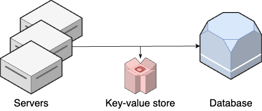
Key-value stores are optimized for a single use case: fast lookup by a known identifier (key). They are effectively a hash table that is distributed across multiple servers. The idea is to deploy the key-value store between your app servers and your primary data store, as shown in Figure 82, so requests that are in the cache (a cache hit) are returned quickly, without having to talk to the primary data store, and only requests that aren’t in the cache (a cache miss) go to the primary data store (after which they are added to the cache to speed up future requests).
Some of the major players in the key-value store space include Redis / Valkey (Valkey is a fork of Redis that was
created after Redis switched from an open source license to dual-licensing) and Memcached
(full list). The API for
most key-value stores primarily consists of just two types of functions, one to insert a key-value pair and one to look
up a value by key. For example, with Redis, you use SET to insert a key-value pair and GET to look up a key:
$ SET key value

OK

$ GET key

value
Key-value stores do not require you to define a schema ahead of time (sometimes referred to as schemaless, but this is a misnomer, as you’ll learn later in this blog post), so you can store any kind of value you want. Typically, the values are either simple scalars (e.g., strings, integers) or blobs that contain arbitrary data that is opaque to the key-value store. Since the data store is only aware of keys and basic types of values, other than operations by primary key, functionality is typically limited. That is, you shouldn’t expect support for flexible queries, joins, foreign key constraints, ACID transactions, or many of the other powerful features of a relational database.
|
Key takeaway #4
Use key-value stores to cache data, speeding up queries and reducing load on your primary data store. |
You can deploy key-value stores yourself, or you can use managed services, such as Redis Cloud and Amazon ElastiCache (full list). Once you have a key-value store deployed, many libraries can automatically use them for cache-aside and write-through caching without you having to implement those strategies manually: e.g., Redis and Memcached plugins for WordPress; Redis Smart Cache plugin for any database you access via JDBC (Java Database Connectivity) APIs.
Let’s now look at the second type of data store commonly used for caching, CDNs.
CDNs
A content delivery network (CDN) consists of servers that are distributed all over the world, called Points of Presence (PoPs), that cache data from your origin servers (i.e., your app servers), and serve that data from a PoP that is as close to the user as possible. Whereas a key-value store goes between your app servers and your database, a CDN goes between your users and your app servers, as shown in Figure 83.
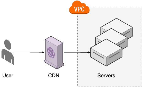
When a user makes a request, it first goes to the PoP that is closest to that user, and if the content is already cached, the user gets a response immediately. If the content isn’t already cached, the PoP forwards the request to your origin servers, caches the response (to make future requests fast), and then returns it to the user. Some of the major players in the CDN space include CloudFlare, Akamai, Fastly, and Amazon CloudFront (full list). CDNs offer several advantages:
- Reduce latency
-
CDN servers are distributed all over the world: e.g., Akamai has more than 4,000 PoPs in over 130 countries. This allows you to serve content from locations that are closer to your users, which can significantly reduce latency (refer back to Table 10), without your company having to invest the time and resources to deploy and maintain app servers all over the world.
- Reduce load
-
Once the CDN has cached a response for a given key, it no longer needs to send a request to the underlying app server for that key—at least, not until the data in the cache has expired or been invalidated. If you have a good cache hit ratio (the percentage of requests that are a cache hit), this can significantly reduce the load on the underlying app servers.
- Improve security
-
Many CDNs provide additional layers of security, such as a web application firewall (WAF), which can inspect and filter HTTP traffic to prevent certain types of attacks (e.g., SQL injection, XSS), and Distributed Denial-of-Service (DDoS) protection, which shields you from malicious attempts to overwhelm your servers with artificial traffic generated from servers around the world.
- Other benefits
-
CDNs have gradually been offering more and more features that let you take advantage of their massively distributed network of PoPs. Here are just a few examples: edge-computing, where the CDN allows you to run small bits of code on the PoPs, as close to your users (as close to the "edge") as possible; compression, where the CDN automatically uses algorithms such as Gzip or Brotli to minimize bandwidth usage; localization, where knowing which local PoP was used allows you to choose the language in which to serve content.
CDNs are most valuable for content that (a) is the same for all of your users and (b) doesn’t change often. For example, news publications can usually offload a huge portion of their traffic to CDNs, as once an article is published, every user sees the same content, and that content isn’t updated too often. On the other hand, social networks and collaborative software can’t leverage CDNs as much, as every user sees different content, and the content changes often.
|
Key takeaway #5
Use CDNs to cache static content, reducing latency for your users and reducing load on your servers. |
One place where virtually all companies can benefit from a CDN is when serving completely static content, such as images, videos, binaries, JavaScript, and CSS. Instead of having your app servers waste CPU and memory on serving up static content, you can offload most of this work to a CDN. In fact, many companies choose not to have their app servers involved in static content at all, not even as an origin server for a CDN, and instead offload all static content to dedicated file servers and object stores, as described in the next section.
File Storage: File Servers and Object Stores
One type of data most companies have to deal with comes in the form of static files. Some of these are files created by your company’s developers, such as the JavaScript, CSS, and images you use on a website. Some of these are files created by your customers, such as the photos and videos users might upload to a social media app. You could store static files in a typical database (e.g., as a blob), which has the advantage of keeping all your data in a single system where you already have security controls, data backups, monitoring, and so on, but using a database for static content also has many disadvantages:
- Slower database
-
Storing files in a database bloats the size of the database, making everything slower. Databases are already a common bottleneck to scalability and availability (as you’ll learn later in this blog post); storing files in them only makes that worse.
- Slower and more expensive replicas and backups
-
Replicating and backing up a larger database is more expensive and slower.
- Increased latency
-
Serving files from your database to a web browser requires you to proxy each file through an app server, which increases latency.
- CPU, memory, and bandwidth overhead
-
Proxying files in a database through an app server increases bandwidth, CPU, and memory usage, both on the app server and the database.
Instead of storing static files in a database, you typically store and serve them from dedicated file servers or object stores, which are the topics of the next two sections.
File Servers
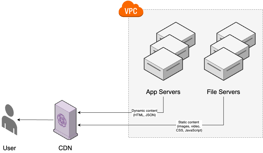
A file server is a server that is designed to store and serve static content, such as images, videos, binaries, JavaScript, and CSS, so that your app servers can focus entirely on serving dynamic content (i.e., content that is different for each user and request). Requests first go to a CDN, which returns a response immediately if it is already cached, and if not, the CDN uses your app servers and file servers as origin servers for dynamic and static content, respectively, as shown in Figure 84:
Most web server and load balancer software can easily be configured to serve files, including all the ones you saw in Part 3 (e.g., Apache, Nginx, HAProxy). The hard part is handling the following:
- Storage
-
You need to provide sufficient hard drive capacity to store the files.
- Metadata
-
You typically need to store metadata related to the files, such as owner, upload date, tags, and so on. You could store the metadata on the file system next to the files themselves, but the more common approach is to store it in a separate data store (e.g., a relational database) that makes it easier to query the metadata.
- Security
-
You need to control who can can create, read, update, and delete files. You may also need to encrypt data at rest and in transit, as you learned in Part 8.
- Scalability and availability
-
You could host all the files on a single server, but as you know from Part 3, a single server is a single point of failure. To support a lot of traffic, and to be resilient to outages, you typically need to use multiple servers.
Solving these problems for a small number of files can be straightforward, but if you get to the scale of a Snapchat, where users upload more than 4 billion pictures per day, these become considerable challenges that require lots of custom tooling, huge numbers of servers and hard drives, RAID, NFS, and so on. One way to make these challenges easier is to offload much of this work to an object store, as discussed in the next section.
Object Stores
An object store (sometimes called a blob store) is a system designed to store opaque objects or blobs, often in the form of files with associated metadata. Typically, these are cloud services, so you can think of object stores as a file server as a service. Some of the major players in this space are Amazon Simple Storage Service (S3), Google Cloud Storage (GCS), and Azure Blog Storage (full list). Object stores provide out-of-the-box solutions to the challenges you saw with file servers in the previous section:
- Storage
-
Object stores provide nearly unlimited disk space, usually for low prices: e.g., Amazon S3 is around $0.02 per GB per month, with a generous free tier.
- Metadata
-
Most object stores allow you to associate metadata with each file you upload: e.g., S3 allows you to configure both system-defined metadata (e.g., standard HTTP headers such as entity tag and content type, as you’ll see later in this blog post) and user-defined metadata (arbitrary key-value pairs).
- Security
-
Most object stores offer access controls and encryption: e.g., S3 provides IAM for access control, TLS for encryption in transit, and AES for encryption at rest.
- Scalability and availability
-
Object stores typically provide scalability and availability at a level few companies can achieve: e.g., S3 provides 99.999999999% durability and 99.99% availability.
Many object stores also provide a variety of other useful features, such as automatic archival or deletion of older files, replication across data centers in different regions, search and analytics[36], integration with compute[37], and more. This combination of features is why even companies who otherwise keep everything on-prem often turn to the cloud and object stores for file storage.
|
Key takeaway #6
Use file servers and object stores to serve static content, allowing your app servers to focus on serving dynamic content. |
To get a better sense for file storage, let’s go through an example.
Example: Serving Files With S3 and CloudFront
In this section, you’re going to set up scalable, highly available, globally-distributed static content hosting by going through the following three steps:
-
Create an S3 bucket configured for website hosting
-
Upload static content to the S3 bucket
-
Deploy CloudFront as a CDN in front of the S3 bucket
Let’s start with creating the S3 bucket.
Create an S3 bucket configured for website hosting
Head into the folder you’ve been using for this blog post series’s examples, and create a folder for a new OpenTofu
root module called static-website:
$ cd fundamentals-of-devops

$ mkdir -p ch9/tofu/live/static-website

$ cd ch9/tofu/live/static-website
You can deploy a website on S3 using a module called s3-website, which is
in the blog post series’s sample code repo in the ch9/tofu/modules/s3-website folder.
The s3-website module creates an S3 bucket, makes its contents publicly accessible, and configures it as a website,
which means it can support redirects, error pages, and so on. To use the s3-website module, create
a file called main.tf in the static-website module, with the contents shown in Example 160:
provider "aws" {

  region = "us-east-2"

}


module "s3_bucket" {

  source  = "brikis98/devops/book//modules/s3-website"

  version = "1.0.0"


  # TODO: fill in your own bucket name!

  name           = "fundamentals-of-devops-static-website" (1)

  index_document = "index.html"                            (2)

}
The preceding code will create an S3 bucket configured as follows:
| 1 | The name to use for the S3 bucket. S3 bucket names must be globally unique, so you’ll have to fill in your own bucket name here. |
| 2 | The suffix to use for directory requests. For example, if you set this to index.html, a request for the directory /foo will return the contents of /foo/index.html. |
Now that you have an S3 bucket, let’s put some content in it, as per the next section.
Upload static content to the S3 bucket
As an example of static content, let’s create an HTML page that includes CSS and an image. First, create a content folder within the static-website folder:
$ mkdir -p contentIn this folder, create index.html with the contents shown in Example 161:
<html lang="en">

  <head>

    <title>Fundamentals of DevOps and Software Delivery</title>

    <link rel="stylesheet" href="styles.css">

  </head>

  <body>

    <h1>Hello, World!</h1>

    <p>This is a static website hosted on S3, with CloudFront as a CDN.</p>

    <img src="cover.png" alt="Fundamentals of DevOps and Software Delivery">

  </body>

</html>
This is a simple HTML page that renders an image and is decorated with a stylesheet. Add an image of your choice into the content folder, naming it cover.png. For the stylesheet, create styles.css with the contents shown in Example 162:
html {

    max-width: 70ch;

    margin: 3em auto;

}


h1, p {

    color: #1d1d1d;

    font-family: sans-serif;

}
Next, update main.tf to upload this content into the S3 bucket as shown in Example 163:
resource "aws_s3_object" "content" {

  for_each = {                                   (1)

    "index.html" = "text/html"

    "styles.css" = "text/css"

    "cover.png"  = "image/png"

  }


  bucket        = module.s3_bucket.bucket_name   (2)

  key           = each.key                       (3)

  source        = "content/${each.key}"          (4)

  etag          = filemd5("content/${each.key}") (5)

  content_type  = each.value                     (6)

  cache_control = "public, max-age=300"          (7)

}
This code uses the aws_s3_object resource to upload files as follows:
| 1 | Have the aws_s3_object resource loop over a map where the key is a file to upload from the content folder and
the value is the content type for that file. |
| 2 | Upload the files to the S3 bucket you created earlier. |
| 3 | For each file, use the key in the map as its path within the S3 bucket. |
| 4 | Read the contents of each file from the content folder. |
| 5 | Set the entity tag (ETag) HTTP response header to the MD5 hash of each file’s contents. This tells web browsers if a file has changed and should be redownloaded. OpenTofu also uses this value to know if a file needs to be reuploaded. |
| 6 | Set the content type HTTP response header for each file to the value in the map. This tells web browsers how to
display the contents of the file: e.g., browsers know to render text/html as HTML, image/png as a PNG image,
and so on. |
| 7 | Set the cache control HTTP response header for each file. The public directive indicates that it’s safe for
shared caches (e.g., CDNs) to cache this resource, while max-age=300 indicates that shared caches and web browsers
can cache this content for up to 300 seconds (5 minutes). |
|
Watch out for snakes: don’t upload files to S3 using OpenTofu
I don’t recommend the |
Finally, add output variables in outputs.tf as shown in Example 164:
output "s3_website_endpoint" {

  description = "The endpoint for the website hosted in the S3 bucket"

  value       = module.s3_bucket.website_endpoint

}
Deploy this code as usual, authenticating to AWS, and running init and apply:
$ tofu init

$ tofu apply
When apply completes, you should see the s3_website_endpoint output. Open http://<S3_WEBSITE_ENDPOINT>;
(S3 websites only support HTTP; CloudFront supports HTTPS, as you’ll see shortly), and you’ll see something like
Figure 85:
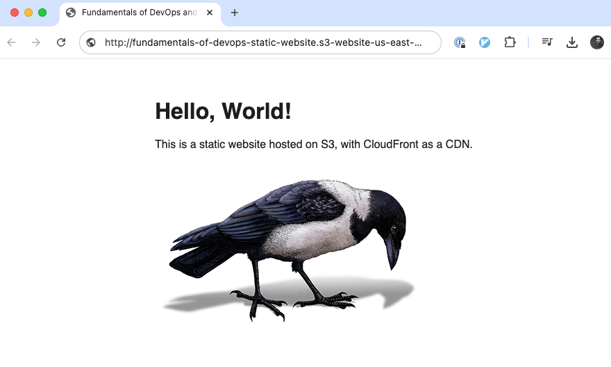
If the page shows up correctly, then congrats, you’re successfully using S3 as a file server! Let’s now put a CDN in front of it, as per the next section.
Deploy CloudFront as a CDN in front of the S3 bucket
To deploy CloudFront as a CDN, you can use a module called cloudfront-s3-website, which is in the blog post series’s
sample code repo in the ch9/tofu/modules/cloudfront-s3-website folder.
The cloudfront-s3-website module creates a globally-distributed CloudFront distribution, configures your static
website in S3 as an origin, sets up a domain name and TLS certificate, and plugs in some basic caching settings.
Update main.tf to use the cloudfront-s3-website module as shown in Example 165:
module "cloudfront" {

  source  = "brikis98/devops/book//modules/cloudfront-s3-website"

  version = "1.0.0"


  bucket_name             = module.s3_bucket.bucket_name      (1)

  bucket_website_endpoint = module.s3_bucket.website_endpoint (2)


  min_ttl     = 0                                             (3)

  max_ttl     = 300

  default_ttl = 0


  default_root_object = "index.html"                          (4)

}
The preceding code configures CloudFront as follows:
| 1 | Pass in the S3 bucket name. This is mostly used as the unique ID within the CloudFront distribution. |
| 2 | Pass in the S3 bucket website endpoint. CloudFront will use this as the origin, sending requests to it for any content that isn’t already cached. |
| 3 | The time-to-live (TTL) settings tell CloudFront how long it should cache content before sending a new request to the origin server (the S3 bucket). The preceding code sets the minimum and default TTL to 0, which tells CloudFront to configure caching based on the content headers (e.g., cache control), and the maximum TTL to 300 seconds (5 minutes), which tells CloudFront not to cache anything longer than that, regardless of headers (which is convenient for testing). |
| 4 | Configure CloudFront to return the contents of index.html whenever someone makes a request to the root of your CloudFront distribution’s domain name. |
Add the CloudFront distribution’s domain name as an output variable in outputs.tf, as shown in Example 166:
output "cloudfront_domain_name" {

  description = "The domain name of the CloudFront distribution"

  value       = module.cloudfront.domain_name

}
Re-run init and apply:
$ tofu init

$ tofu apply
CloudFront can take 2-10 minutes to deploy, so be patient. When apply completes, you should see the
cloudfront_domain_name output variable. Open https://<CLOUDFRONT_DOMAIN_NAME>; (yes, HTTPS this time!) in your web
browser, and you should see the same content as Figure 85. Congrats, you’re now serving and caching
static content via a network of 600+ CloudFront PoPs dispersed all over the world!
|
Get your hands dirty
Here are a few exercises you can try at home to go deeper:
|
When you’re done testing, commit your changes to Git, and run tofu destroy to clean everything up again. Now that
you’ve seen how to store files, let’s turn our attention to the next use case, which is handling semi-structured data
and search.
Semi-Structured Data and Search: Document Stores
Relational databases are a great choice when your data has a clear, consistent, and predictable structure, which allows you to store the data in tables with well-defined schemas, and perform queries on well-defined column names. However, this isn’t always the case. For example, if you are building software similar to a wiki, where users can create arbitrary documents, tags, categories, labels, and so on, it may be tough to fit all this into a static relational schema. For these use cases, where you are dealing with semi-structured data, a document store may be a better fit. A document store is similar to a key-value store, except the values are richer data structures called documents that the document store natively understands, so you get access to more advanced functionality for querying and updating that data.
Popular general-purpose document stores include MongoDB and Couchbase (full list). There are also document stores that are optimized for search: that is, building search indices on top of the documents, so you can use free-text search, faceted search, and so on. Some of the popular options for search include Elasticsearch / OpenSearch (OpenSearch is a fork of Elasticsearch that was created after Elasticsearch switched from an open source license to dual-licensing), and Algolia (full list).
The next several sections will take a brief look at document stores by considering the same data storage concepts you saw with relational databases:
-
Reading and writing data
-
ACID Transactions
-
Schemas and constraints
We’ll start with reading and writing data.
Reading and Writing Data
To get a sense of how document stores work, let’s use MongoDB as an example. MongoDB allows you to store JSON documents
in collections, somewhat analogously to how a relational database allows you to store rows in tables. MongoDB does
not require you to define a schema for your documents, so you can store JSON data in any format you want. To read and
write data, you use the MongoDB Query Language (MQL), which is similar to JavaScript. Example 167
shows how you can use the insertMany command to store JSON documents in a collection called bank:
bank collection (ch9/mongodb/bank.js)db.bank.insertMany([
{name: "Brian Kim", date_of_birth: new Date("1948-09-23"), balance: 1500},
{name: "Karen Johnson", date_of_birth: new Date("1989-11-18"), balance: 4853},
{name: "Wade Feinstein", date_of_birth: new Date("1965-02-25"), balance: 2150}
]);This is the same bank example you saw with relational databases earlier in this blog post, with the
same three customers as in Table 18. To read data back out, you can use the find command as shown in
Example 168:
bank collection (ch9/mongodb/bank.js)db.bank.find();
[
{
_id: ObjectId('66e02de6107a0497244ec05e'),
name: 'Brian Kim',
date_of_birth: ISODate('1948-09-23T00:00:00.000Z'),
balance: 1500
},
{
_id: ObjectId('66e02de6107a0497244ec05f'),
name: 'Karen Johnson',
date_of_birth: ISODate('1989-11-18T00:00:00.000Z'),
balance: 4853
},
{
_id: ObjectId('66e02de6107a0497244ec060'),
name: 'Wade Feinstein',
date_of_birth: ISODate('1965-02-25T00:00:00.000Z'),
balance: 2150
}
]You get back the exact documents you inserted, except for one new item: MongoDB automatically adds an _id field to
every document, which it uses as a unique identifier, similar to a primary key. For example,
you can look up a document by ID as shown in Example 169:
db.bank.find({_id: ObjectId('66e02de6107a0497244ec05e')});


{

  _id: ObjectId('66e02de6107a0497244ec05e'),

  name: 'Brian Kim',

  date_of_birth: ISODate('1948-09-23T00:00:00.000Z'),

  balance: 1500

}
The big difference between key-value stores and document stores is that document stores can natively understand and process the full contents of each document, rather than treating them as opaque blobs. This gives you richer query functionality. Example 170 shows how you can find all customers born after 1950, the same query you saw in SQL in Example 146:
db.bank.find({date_of_birth: {$gt: new Date("1950-12-31")}});


[

  {

    _id: ObjectId('66e02de6107a0497244ec05f'),

    name: 'Karen Johnson',

    date_of_birth: ISODate('1989-11-18T00:00:00.000Z'),

    balance: 4853

  },

  {

    _id: ObjectId('66e02de6107a0497244ec060'),

    name: 'Wade Feinstein',

    date_of_birth: ISODate('1965-02-25T00:00:00.000Z'),

    balance: 2150

  }

]
You also get richer functionality when updating documents. Example 171 shows
how you can use the updateMany command to deduct $100 from all customers, similar to the SQL UPDATE you saw in
Example 147:
db.bank.updateMany({}, {$inc: {balance: -100}});All of this richer querying and update functionality is great, but there are two major limitations. First, most document stores do not support working with multiple collections: that is, there is no support for joins.[38] Second, most document stores don’t support ACID transactions, as discussed in the next section.
ACID Transactions
There is a serious problem with the code in Example 171: most document stores
don’t support ACID transactions.[39] You might get atomic operations on a single document (e.g., if you
updated one document with the updateOne command), but you rarely get it for updates to multiple documents. That means
it’s possible for that code to deduct $100 from some customers but not others: e.g., if MongoDB crashes in the middle
of the updateMany operation.
This is not at all obvious from the code, and many developers who are not aware of this are caught off guard when their document store operations don’t produce the results they expect. This is one of many gotchas with using non-relational databases, especially as your source of truth. Other major gotchas include dealing with eventual consistency, as you’ll see later in this blog post, and the lack of support for schemas and constraints, as discussed in the next section.
Schemas and Constraints
Most document stores do not require you to define a schema or constraints up front. This is sometimes referred to as
schemaless, but that’s a bit of a misnomer. The reality is that there is always a schema. The only
question is whether you enforce a schema-on-read or a schema-on-write. Relational databases enforce a schema-on-write,
which means the schema and constraints must be defined ahead of time, and the database will only allow you to write
data that matches the schema and constraints. Most document stores, such as MongoDB, don’t require you to define the
schema or constraints ahead of time, so you can structure your data however you want, but eventually, something will
read that data, and that code will have to enforce a schema-on-read to be able to parse the data and do something
useful with it. For example, to parse data from the bank collection you saw in the previous section, you might create
the Java code shown in Example 172:
public class Customer {

    private String name;

    private int balance;

    private Date dateOfBirth;

}
The Java class in Example 172 defines a schema and constraints: i.e., you’re expecting field names such
as name and balance with types String and int, respectively. More accurately, this is an example of
schema-on-read, as this class defines the schema you’re expecting from the data store, and either the data you read
matches the Customer data structure, or you will get an error. Since document stores don’t enforce schemas or
constraints, you can insert any data you want in any collection, such as the example shown in
Example 173:
db.bank.insertOne(

  {name: "Jon Smith", birth_date: new Date("1991-04-04"), balance: 500}

);
Did you catch the error? The preceding code uses birth_date instead of date_of_birth. Whoops. MongoDB will
allow you to insert this data without any complaints, but when you try to parse this data with the Customer class,
you may get an error. And this is just one of many types of errors you may get with schema-on-read. Since most document
stores don’t support domain constraints or foreign key constraints, you will also have to worry about typos in field
names, incorrect types for fields, IDs that reference non-existent documents in other collections, and so on.
Dealing with these errors when you read the data is hard, so it’s better to prevent these errors in the first place by blocking invalid data on write. That’s an area where schema-on-write has a decided advantage, as it allows you to ensure your data is well-formed by enforcing a schema and constraints in one place, the (well-tested) data store, instead of trying to enforce it in dozens of places, including in every part of your application code, every script, every console interaction, and so on.
That said, schema-on-read is advantageous if you are dealing with semi-structured or non-uniform data. I wouldn’t use a document store for highly structured bank data, but I might use one for user-generated documents, event-tracking data, and log messages. Schema-on-read can also be advantageous if the schema changes often. With a relational database, certain types of schema changes take a long time or even require downtime. With schema-on-read, all you have to do is update your application code to be able to handle both the new data format and the old one, and your migration is done. Or, to be more accurate, your migration has just started, and it will happen incrementally as new data gets written.
|
Key takeaway #7
Use document stores for semi-structured and non-uniform data, where you can’t define a schema ahead of time, or for search, when you need free-text search, faceted search, etc. |
There’s one other trade-off to consider between schema-on-read and schema-on-write: performance. With schema-on-write, as with a relational database, the data store knows the schema ahead of time, and the schema is the same for all the data in a single table, so the data can be stored efficiently, both in terms of disk space usage, and the performance of disk lookup operations. With schema-on-read, as with a document store, since each document can have a different schema, the data store has to store the schema with that document, which is less efficient. This is one of the reasons that data stores that are designed for performance and efficiency typically use schema-on-write. This includes data stores designed to extract insights from your data using analytics, as discussed in the next section.
Analytics: Columnar Databases
There are a number of data storage technologies that are optimized for storing your data in a format that makes it easier and faster to analyze that data. This is part of the larger field that is now called data science, which combines statistics, computer science, information science, software engineering, and visualization to extract insights from your data. A deep dive on data science is beyond the scope of this blog post series, but it is worth briefly touching on some of the data storage technologies that are involved, as deploying and maintaining these systems often falls under the purview of DevOps.
Under the hood, many analytics systems are based on columnar databases, so the next section will go through the basics of what a columnar database is, and the section after that will look at common columnar database use cases.
Columnar Database Basics
On the surface, columnar databases (AKA column-oriented databases) look similar to relational databases, as
they store data in tables that consist of rows and columns, they usually have you define a schema ahead of time, and
sometimes, they support a query language that looks similar to SQL. However, there are a few major differences.
First, most columnar databases do not support ACID transactions, joins, foreign key constraints, and many other key
relational database features. Second, the key design principle of columnar databases, and the source of their name,
is that they are column-oriented, which means they are optimized for operations across columns, whereas relational
databases are typically row-oriented, which means they are optimized for operations across rows of data. This is best
explained with an example. Consider the books table shown in Table 19:
| id | title | genre | year_published |
|---|---|---|---|
1 |
Clean Code |
tech |
2008 |
2 |
Code Complete |
tech |
1993 |
3 |
The Giver |
sci-fi |
1993 |
4 |
World War Z |
sci-fi |
2006 |
How does this data get stored on the hard drive? In a row-oriented relational database, the values in each row will be kept together, so conceptually, the serialized data might look similar to what you see in Example 174:
[1] Clean Code,tech,2008

[2] Code Complete,tech,1993

[3] The Giver,sci-fi,1993

[4] World War Z,sci-fi,2006
Compare this to the way a column-oriented store might serialize the same data, as shown in Example 175:
[title] Clean Code:1,Code Complete:2,The Giver:3,World War Z:4

[genre] tech:1,2,sci-fi:3,4

[year_published] 2008:1,1993:2,3,2006:4
In this format, all the values in a single column are laid out sequentially, with the contents of a column as keys
(e.g., Clean Code or tech), and the IDs as values (e.g., 1 or 1,2). Now consider the query shown in
Example 176:
SELECT * FROM books WHERE year_published = 1993;


 id |     title     | genre  | year_published

----+---------------+--------+----------------

  2 | Code Complete | tech   |           1993

  3 | The Giver     | sci-fi |           1993
Because this query uses SELECT *, it will need to read every column for any matching rows. With the row-oriented
storage in Example 174, the data for all the columns in a row is laid out sequentially on the hard
drive, whereas with the column-oriented storage in Example 175, the data for each column is
scattered across the hard drive. Hard drives perform better for sequential reads than random reads, so for this sort of
query, especially with a large amount of data (think millions or billions of rows), the row-oriented approach will be
considerably faster. Compare that to the query in Example 177:
SELECT COUNT(*) FROM books WHERE year_published = 1993;


 count

-------

     2
This query uses an aggregate, SELECT COUNT(*), so it will only need to read the values in the year_published column
to satisfy the WHERE clause, and then count how many matches there are. With the row-oriented storage in
Example 174, this requires jumping all over the hard drive to read the year_published value for
each row, whereas with the column-oriented storage in Example 175, all the data for the
year_published column is laid out sequentially, so for this sort of query, with millions or billions of rows, the
column-oriented approach will be considerably faster. When you’re doing analytics, aggregate functions such as
COUNT, SUM, AVG come up all the time, which is why the column-oriented approach is used in a large number of
analytics use cases, as described in the next section.
Analytics Use Cases
The following are some of the most common use cases for columnar databases:
- General-purpose columnar databases
-
Popular columnar databases that you can use for a wide variety of use cases include Cassandra, Google Bigtable, and HBase (full list).
- Time-series databases
-
Many data stores that are designed for storing and analyzing time-series data, such as metrics and logs, also use column-oriented designs, as it’s common to perform aggregate queries on this sort of data (e.g., show me the average response time for my app). Popular time-series databases include Prometheus and InfluxDB (full list).
- Big data
-
Big data is a somewhat fuzzy term that relates to data sets that are vastly larger than what you can process using traditional data analytics systems, such as relational databases, document stores, and so on. This is a significant challenge for companies operating at massive scale, such as Google, Facebook, Twitter, and so on. In 2004, Google released a paper on MapReduce, which described their approach to batch processing huge amounts of data using distributed systems. This kicked off a wave of big data tools. Some of the major players in this space include Hadoop (an open source MapReduce implementation) and Cloudera (full list).
- Fast data
-
Big data systems typically do batch processing, generating analytics from large data sets by running in the background on a periodic basis (e.g., once per day). Fast data systems are designed to do stream processing (a topic you’ll learn more about later in this blog post), generating analytics from large data sets by running continuously, incrementally processing streams of data on a near real-time basis (e.g., in milliseconds). Some of the major players in this space include Apache Spark and Apache Flink (full list).
- Data warehouses
-
A data warehouse is a central repository where you integrate data from all of your other systems, as shown in Figure 86. With all of your data in one place, you can perform a variety of analytics, generate reports, and so on. Data warehouses are often column-oriented, and use specialized schemas (e.g., star and snowflake schemas) optimized for analytics. Some of the major players in the data warehouse space include Snowflake, Amazon Redshift, and Google BigQuery (full list).
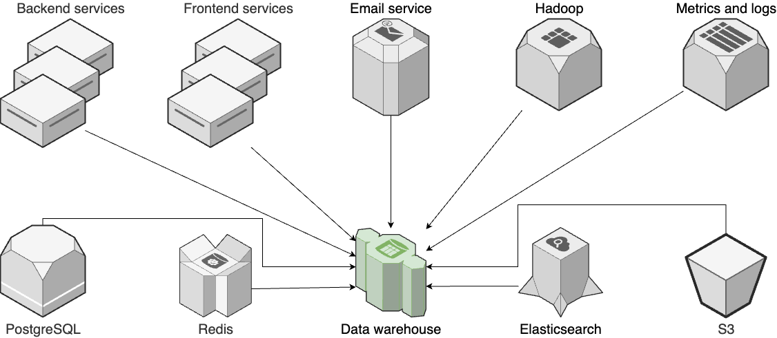 Figure 86. Integrating all your data in a data warehouse
|
Key takeaway #8
Use columnar databases for time-series data, big data, fast data, data warehouses, and anywhere else you need to quickly perform aggregate operations on columns. |
The diagram in Figure 86 is highly simplified. First, what look like simple arrows from the various systems to the data warehouse are actually complicated background processes known as extract, transform, and load (ETL) that extract data from one system in one format, transform it into the format used by another system (cleaning up and standardizing the data along the way), and then load it into that other system. This is complicated enough that a whole ecosystem of ETL tools has sprung up, including Apache Airflow, Stitch, and Qlik (full list). Second, there are not only arrows from each system to the data warehouse, but arrows between many of the other systems, too, representing background jobs, event-based communication, and so on. All of this falls into the realm of asynchronous processing, which is the topic of the next section.
Asynchronous Processing: Queues and Streams
In Part 7, you learned about how microservices can communicate with each other using tools such as service discovery and service meshes. This approach typically uses synchronous communication, where service A sends a request to service B and waits for service B to send a response before moving on. There are also many use cases where you want to use asynchronous communication, where a service A sends a message to service B, and then moves on without waiting for the response. Service B can process that message at its own pace, and if it needs to send a response, it can send a new asynchronous message to service A.
Note that there is a hidden implication in the asynchronous style of communication: you want to be sure that each message is (eventually) processed. Losing a message or processing it multiple times could have negative consequences for your business. Therefore, you don’t typically just send these messages from service A directly to service B, and have service B hold on to the message in memory, as (a) depending on the number of messages, this could use up more memory than service B has available and (b) if service B crashes, then all messages it hasn’t processed will be lost. Instead, service A sends messages to, and service B reads messages from, a data store that is designed to facilitate this type of asynchronous communication by persisting messages to disk and tracking the state of those messages (e.g., whether they have been processed). Broadly speaking, there are two types of data stores that can do this:
-
Message queues
-
Event streams
The next two sections will dive into each of these, starting with message queues.
Message Queues
A message queue is a data store that can be used for asynchronous communication between producers, who write messages to the queue, and consumers, who read messages from the queue, as shown in Figure 87.
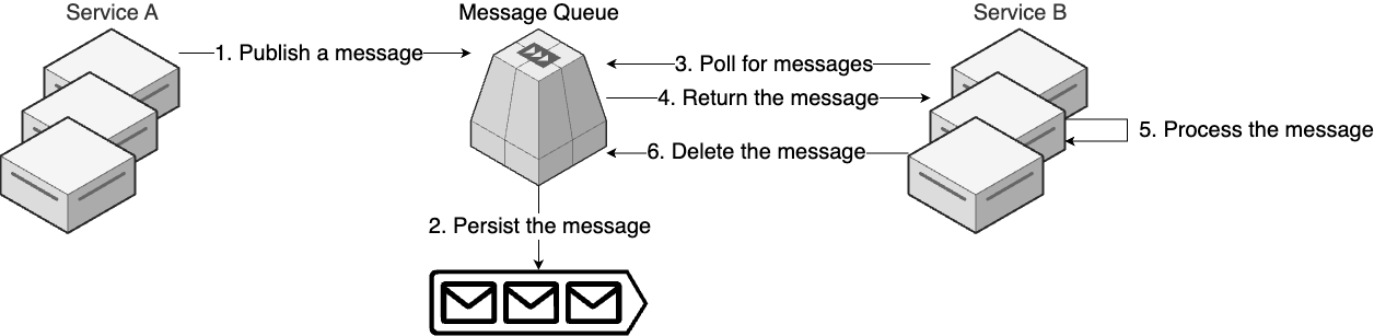
The typical process of using a queue is:
-
A producer, such as service A, publishes a message to the queue.
-
The queue persists the message to disk. This ensures the message will eventually be processed, even if the queue or either service has an outage.
-
A consumer, such as service B, periodically polls the queue for new messages.
-
When there is a new message, the queue returns the message to service B. The queue may record that the message is "in progress" so that no other consumer can read the message at the same time.
-
Service B processes the message.
-
Once the message has been successfully processed, service B deletes the message from the queue. This ensures that the message is only processed one time.
Queues are most often used for tasks that run in the background, as opposed to tasks you do during a live request from a user. For example, if you are building an app that lets users upload images, if you need to process each image (e.g., create copies of the image in different sizes for web, mobile, thumbnail previews, etc.), you may want to do that in the background, rather than making the user wait for it. To do that, your frontend server stores the original image on a file server and adds a message to a queue with the location of the image. Later on, a separate consumer process reads the message from the queue, downloads the image from the file server, processes the image, and when it’s done, deletes the message from the queue. Other common use cases include encoding videos, sending email campaigns, delivering notifications, generating reports, and order processing.
Some popular message queues include RabbitMQ, ActiveMQ, and ZeroMQ (full list). Queues provide several key benefits:
- Handle traffic spikes
-
A queue acts as a buffer between your services, which allows you to deal with spikes in traffic. If service A and B were communicating synchronously, and traffic suddenly increased by 10x, then B might not be able to keep up with the load, and you’d have outages and lost messages. With the queue in between, service A can write as many messages as it wants, and service B can process them at whatever rate it can handle.
- Decoupling
-
With synchronous communication, every service needs to know the interface to talk to every other service. In a large company, one service may use JSON over HTTP whereas another uses gRPC; one service may be in a service mesh that requires mTLS, while another is a legacy service that is not in the mesh; and so on. Connecting many disparate services can be a massive undertaking. With asynchronous communication via a message queue, each service solely needs to know how to talk to one thing, the API used by the message queue, so it gives you a decoupled, standardized mechanism for communication.
- Guarantee tasks are completed
-
If service A sends a synchronous message to service B, but never gets a response, or gets an error, what do you do? Most code just errors out. Some code uses retry logic, but if you’re not careful, this might result in service B processing the message multiple times, or, if service B is overloaded, it might make the problem worse. Using asynchronous communication with a message queue allows you to guarantee that each task is (eventually) completed, even in the face of outages and crashes, as the queue persists message data and metadata (e.g., whether that message has been processed). Note that in distributed systems theory, guaranteeing a message is delivered exactly once is provably impossible (if you’re curious why, look up the Two Generals Problem), so in practice, most message queues provide at least once delivery, and you create consumers who are idempotent (i.e., can ignore duplicate messages).
- Guarantee ordering and priority
-
Some message queues can guarantee not only at least once delivery, but also that messages are delivered in a specific order, such as first-in, first out (FIFO) queues, which deliver messages in the order they were received, and priority queues, which deliver messages with the highest priority first.
|
Key takeaway #9
Use message queues to run tasks in the background, with guarantees that tasks are completed and executed in a specific order. |
Whereas message queues are used for one-to-one communication between a producer and a consumer, event streams are used for one-to-many communication, as discussed in the next section.
Event Streams
Event streaming tools allow services to communicate asynchronously in a manner similar to a message queue, but the main difference is that instead of each message being consumed by a single consumer, streaming allows each message to be consumed by multiple consumers, as shown in Figure 88. Some of the most popular event streaming tools include Apache Kafka, Amazon Kinesis, and NATS (full list).
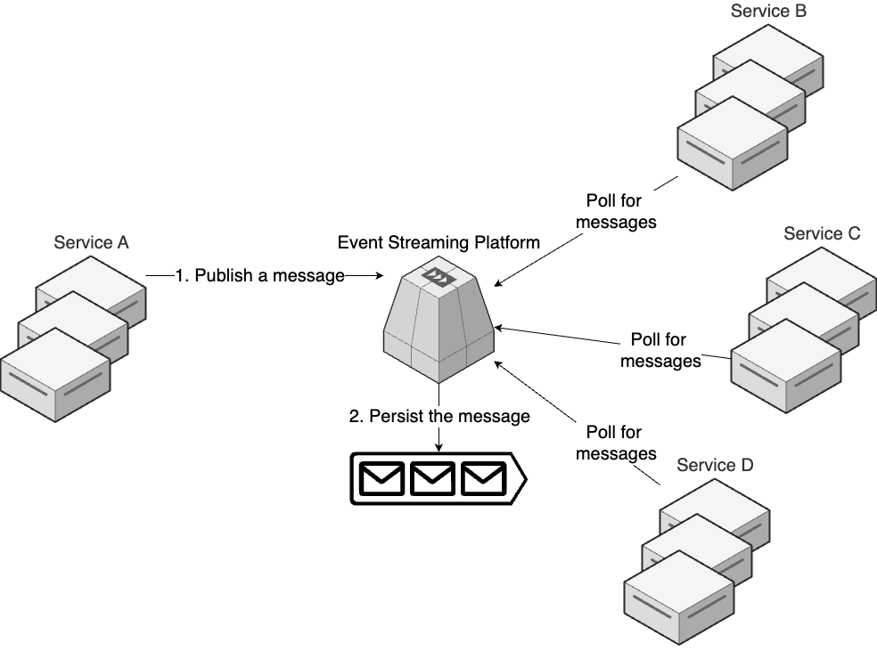
The typical process of using event streaming is:
-
A producer, such as service A, publishes a message to the event stream.
-
The event stream persists the message to disk. This ensures the message will eventually be processed, even if the event stream or any other service has an outage. Under the hood, the messages are recorded in a log, which is an append-only, totally-ordered sequence of records, ordered by time, as shown in Figure 89.
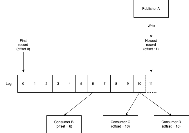 Figure 89. An event streaming log, with one publisher and three consumers
 -
One or more consumers, such as services B, C, and D, polls the event streaming platform for new messages.
-
For each consumer, the streaming platform records that consumer’s offset in the log: that is, the last message that consumer saw. When there is a new message past that offset, the streaming platform returns that message to the consumer.
-
Services B, C, and D process whatever messages they receive.
-
Once a service has successfully processed a message, it updates its offset in the streaming platform log, ensuring it won’t see the same message again.
At its most basic level, event streaming could be used as a replacement for a message queue to allow services to communicate asynchronously, but this is not the primary use case. Whereas a message queue is typically used to allow service A to send a message specifically destined for service B, the idea with event streaming is for every service to publish a stream of events that represent important data points or changes in state in that service, but aren’t necessarily designed for any one specific recipient, which allows for multiple other services to subscribe and react to whatever streams of events are relevant to them. This is known as an event-driven architecture.
The difference between messages in a message queue and events in an event stream has a profound impact on how you build your services. In Figure 86, you saw a simplified diagram showing all systems sending their data to a data warehouse. Figure 90 shows a slightly more realistic image:
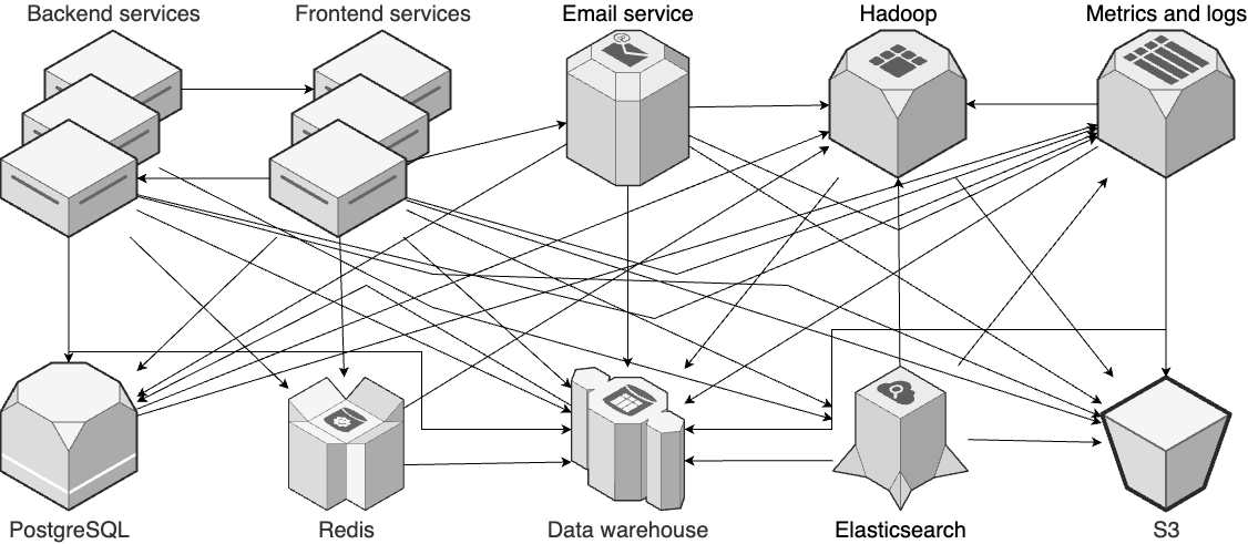
As the number of services grows, the number of connections between them grows even faster. With N services, you end up with roughly N2 connections, across a variety of interfaces and protocols that often require complicated ETL. Setting up and maintaining all these connections can be a massive undertaking. Event streaming offers an alternative solution, as shown in Figure 91:
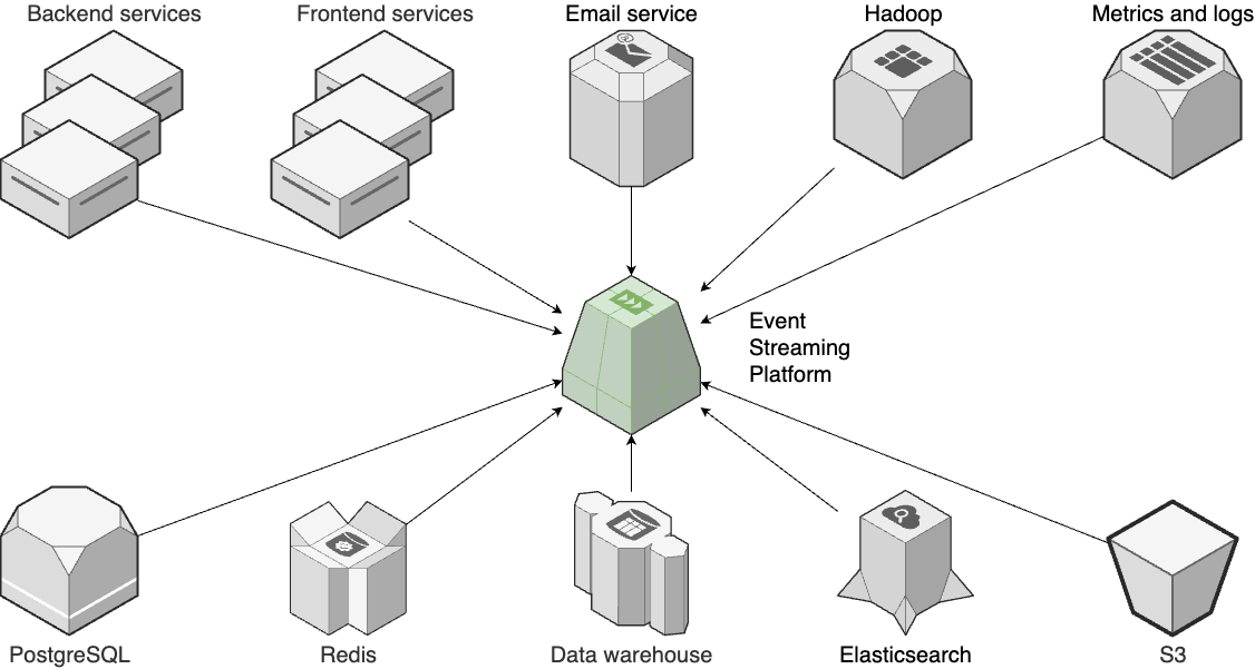
In Part 7, you saw that a network switch allows you to connect N computers with N cables (each computer has one cable connected to the switch) instead of N2. Analogously, an event streaming platform allows you to connect N services with N connections (each service has one connection to the event streaming platform) instead of N2. Dramatically simplified connectivity is one of the major benefits of an event-driven architecture. Another major benefit, and one that’s less obvious, is that an event-driven architecture allows you to add new services—new consumers—without having to modify any existing producers.
An example can help illustrate the power of this concept. First, consider an architecture where services message each other directly. For example, service A might send the message "a new image has been uploaded to location X, please process that image" to service B. 6 months later, you want to add a new service C to scan images for inappropriate content. In order for this service to do its job, you have to update service A to send an additional message to service C: "a new image has been uploaded to location X, please scan that image for inappropriate content."
Now compare this to an event-driven architecture, where service A doesn’t have to know about the existence of other services at all. Service A merely publishes important events, such as "a new image has been uploaded to location X." Perhaps on day one, service B subscribes to this event stream, and is able to process each image; 6 months later, when you add service C, it can subscribe to the same event stream to start scanning images for inappropriate content—without any need to modify service A. You could add dozens more services that consume service A’s event stream, again, with no need for A to be aware of them at all.
In an event-driven architecture, every service publishes important events, such as "a new user has registered," "a user clicked a button," "an order has been placed," "a server is down," and so on. Any other service can subscribe to any of these events streams to perform a variety of actions: e.g., update a search index, detect fraudulent activity, generate a report, send out a notification, and so on. Moreover, each time a service subscribes to an event stream, it can choose to start at offset 0 in that stream (refer to Figure 89), effectively "going back in time," and processing all the historical events from that event stream (e.g., all images that have ever been uploaded) until it catches up to the latest offset, or it can start immediately at the latest offset, and just process new events.
Event-driven architectures provide a large number of benefits:
- All the benefits of a message queue
-
Event streams offer most of the same benefits as you saw with message queues in the previous section: they help you handle traffic spikes, decouple services, guarantee tasks are completed, and guarantee task ordering.
- Even stronger decoupling
-
Message queues provide a limited amount of decoupling by allowing services to communicate by only having to interact with one interface, the queue, but some coupling remains, as each service must be aware of other services to send them messages. Event streaming also allows services to only interact with a single interface, the event streaming platform, but it is even more decoupled, as publishers don’t need to be aware of consumers at all. This unlocks remarkable flexibility and scalability in your architecture.
- Monitoring
-
Event streaming turns out to be an excellent way to implement monitoring, including metrics and logs. The stream of events from each service inherently provides visibility into what that service is doing, and you can hook up various consumers to help make your monitoring data easier to visualize, search, and so on. You’ll learn more about monitoring in Part 10.
- ETL and stream processing
-
In the analytics section earlier in this blog post, you learned about big data, fast data, and data warehouses. Event streams play a key role in each of these. First, event streaming gives you a single, standardize way to do ETL. Second, I mentioned that fast data is all about processing streams of data; well, the event stream platform is what provides those streams of data!
|
Key takeaway #10
Use event streams to build highly-scalable, decoupled, event-driven architectures. |
Let’s now move on to the next section, which focuses not on a specific data storage use case, but on the general problem of data store scalability and availability.
Scalability and Availability
For many companies, the data store is the biggest bottleneck in terms of scalability and availability. It’s relatively easy to make stateless software scalable and highly available; it’s considerably trickier to do so for stateful software. Over the years, there have been many attempts to solve this problem, and the key thing we’ve learned is that there’s no one-size-fits-all solution. No data store or architecture is a silver bullet that can magically fix all your scalability and availability challenges. That said, there are some patterns that come up again and again. The next several sections will look at these common patterns in the following systems:
-
Relational databases
-
NoSQL and NewSQL databases
-
Distributed systems
Let’s start with scalability and availability patterns for relational databases.
Relational Databases
Most relational databases are designed to run on a single server. However, as you learned in Part 3, a single server is a single point of failure—a bottleneck to scalability and availability. This isn’t something you have to worry about until you are storing tremendous amounts of data and serving a huge amount of traffic, but if you get to that point, you should be aware that it’s easy to scale a database vertically by making a single server more powerful (more CPU, more memory, more disk space), but it’s harder to scale a database horizontally across multiple servers. To horizontally scale a relational database—or any data store—there are two primary strategies, replication and partitioning, as discussed in the next two sections.
Replication
Replication involves copying the same data to multiple servers called replicas. One of the key benefits of replication is fault tolerance. Servers and hard drives fail all the time, so having a copy of your data in more than one place can help improve availability. One option is to replicate data to a standby replica, which doesn’t serve any live traffic but can be swapped in quickly if the primary database goes down. Another option is to replicate data to one or more active replicas, which serve live traffic, thereby allowing you to horizontally scale your database by adding more replicas. Note that with a relational database, these are read replicas, which can handle read traffic, whereas all write traffic must instead go to the primary database. This helps you offload all read traffic from the primary database, which is especially helpful for the many types of software that have vastly more reads than writes.
Partitioning
Whereas replication is copying the same data to multiple servers, partitioning (AKA sharding) is copying
different subsets of the data to different servers, where each of those servers can handle both reads and writes. The
goal of partitioning is to divide your data set deterministically between n servers so that each one only has to
handle 1/nth of the total load. Going back once more to the bank example, if you had grown to 10 million customers,
you could partition them across 10 servers, so all the data in the customers table for customers with id 0 -
1,000,000 would be on server 0, all the data for customers 1,000,001 - 2,000,000 would be on server
1, and so on. If the bank had a website where most of the pages only showed data for one customer at a time, then
each database would only have to handle ~10% of the load, which is a huge win.
Partitioning effectively turns a single-node database into a distributed system, which helps with availability and
scalability, but it comes at a cost. We’ll dive into distributed systems challenges later in this
blog post, but for now I’ll list just a few examples. With partitioning, you lose the ability to use
auto-incrementing sequences, queries across data in different partitions, and foreign key constraints across data in
different partitions. You even lose ACID transactions for data in different partitions: e.g., if a customer with id
50 wanted to transfer money to a customer with id 3,000,000, since the data for each customer lives in a separate
partition, you couldn’t perform this update in a single transaction. Moreover, if you don’t partition your data
correctly, or if your access patterns change, it’s possible to develop hot spots, where certain partitions get a
disproportionately higher percentage of traffic and become overloaded. To fix these, you have to update the
partitioning strategy, known as rebalancing, which can be difficult and expensive, as it may require moving a lot of
data around.
|
Key takeaway #11
Use replication and partitioning to make relational databases more scalable and highly available. |
Replication and partitioning can provide a remarkable amount of scalability and availability for a relational database. For example, Meta uses a relational database (MySQL) as the primary data store for its 3+ billion users, and the scale of their deployment is astonishing, consisting of thousands of servers across multiple continents, hosting millions of shards, and storing petabytes of data.[40] That said, some companies choose to handle scalability and availability challenges by moving away from relational databases entirely, as discussed in the next section.
NoSQL and NewSQL Databases
In the mid-to-late 2000s, the challenges with scalability and high availability for relational databases led to the creation of a number of non-relational databases, often called NoSQL databases. NoSQL, which at various times stood for Non-SQL or Not-Only-SQL, is a fuzzy term that refers to databases that do not use SQL or the relational model. Over the years, there have been many types of non-relational databases, most of which failed to gain wide adoption (e.g., object databases in the 90s, XML databases in the early 2000s), but NoSQL in particular refers to databases that were built in the late 2000s, primarily by Internet companies struggling to adapt relational databases to unprecedented demands in performance, availability, and data volume.
The early inspirations for NoSQL included Google’s 2006 paper on BigTable and Amazon’s 2007 paper on Dynamo. The actual term "NoSQL" came after these papers, originating as a Twitter hashtag (#NoSQL) for a 2009 meetup in San Francisco to discuss "open source, distributed, non-relational databases," which is still the best definition of NoSQL that we have. The primary types of data stores that fall under the NoSQL umbrella are key-value stores, document stores, and columnar databases, all of which you’ve already seen in this blog post.[41]
Most NoSQL databases were designed from the ground up for scalability and availability, so the default deployment often includes replication and partitioning. For example, MongoDB is typically deployed in a cluster that consists of multiple shards, where each shard has a primary (for writes) and one or more replicas (for reads), plus dedicated servers that handle query routing, auto-sharding, and auto-rebalancing. The benefit is that you get a highly scalable and available data store. The cost is that these are complicated distributed systems, and that comes with a number of challenges, as you’ll see in the next section. For now, I’ll just say that, in the pursuit of scalability and high availability, most NoSQL data stores sacrifice key features from relational databases, such as ACID transactions, referential integrity, and flexible query languages that support joins.
For some use cases, this was too many sacrifices, which led to the creation of a new breed of relational database in the mid-to-late 2010s, often called NewSQL, that tried to retain the strengths of a relational database (e.g., ACID transactions, SQL), while providing better availability and scalability. Some of the major players in this space include Google Spanner, Amazon Aurora, and CockroachDB (full list). Under the hood, these are also complex distributed systems that use replication and partitioning to achieve high scalability and availability, but they try to use new techniques to not sacrifice too many relational database benefits along the way. The approaches they use are fascinating, but beyond the scope of this blog post series, especially as many of the early NewSQL players died out, and the ones that remain are still relatively young and immature.
Remember, data storage technology takes at least a decade to mature. As of the writing of this blog post series, most NoSQL data stores are 10-15 years old, so they are just starting to become mature and reliable systems. Most NewSQL systems are still less than 10 years old, so they are still relatively young (at least as far as data storage technologies go). Given that both NoSQL and NewSQL databases are typically complex distributed systems, they face challenges that may take even more than a decade to solve, as discussed in the next section.
Distributed Systems
As you may remember from Part 6, distributed systems are complicated, and distributed data stores even more so. One of the challenges is that all distributed systems are subject to the CAP theorem, which gets its name from the following three properties:
- Consistency (C)
-
Every read receives the most recent write.
- Availability (A)
-
Every request receives a response, even if some servers are down.
- Partition tolerance (P)
-
The distributed system continues to work even if there is a break in communications (known as a partition) between some of the servers.
All three of these are desirable properties for a distributed system, but the CAP theorem says you can only pick two. Moreover, in practice, no network can guarantee there will never be any partitions, so all real-world distributed systems have to provide partition tolerance—they have to pick P—which means you really only get to pick one more. That is, in the presence of a network partition, does your distributed system provide consistency (C) or availability (A)?
Some systems, such as HBase and Redis, pick C, so they try to keep data consistent on all nodes, and in the case of a network partition, they lose availability. If you use a data store that picks C, you have to accept that, from time to time, that data store will be down. Other systems, such as Cassandra, Riak, and CouchDB, pick A, so they are eventually consistent, which means that during a network partition, they will remain available, but different nodes may end up with different data. In fact, even without a partition, eventually consistent systems may have different data on different nodes, at least for a short amount of time. If you use a data store that picks A, then you have to deal with an eventually consistent data model, which can be confusing for programmers and users (e.g., you just updated some data, but after refreshing the page, you still see the old data). Some systems, such as MongoDB, allow you to tune for availability or consistency via configuration settings, allowing you to pick C or A depending on the use case.
Another challenge with distributed systems is that they introduce many new failure modes. At some point, every data store will fail. The question is, how many different ways can the system fail and how easy is it to understand and fix each one? Usually, the number and complexity of failure modes on a single-node system (e.g., a relational database) is far lower than on a distributed NoSQL or NewSQL system that has multiple writers, auto-sharding, auto-rebalancing, eventual consistency, consensus algorithms, and so on. Having to deal with too many failure modes was one of the main reasons Pinterest stopped using Cassandra and Etsy stopped using MongoDB.
One more challenge with distributed systems is figuring out a business model to support them. It takes a decade or two to build a reliable data store, and finding a way to sustainably pay developers during all that time is tricky. Many data store companies have shut down—e.g., RethinkDB, FoundationDB, GenieDB, ScaleDB, and many others—which is a huge problem if your company relies on these technologies for storing your most valuable asset! A data store that has been around 20+ years is not only more mature than a data store that just came out in the last few years, but it’s also more likely than the new data store to still be around another 20 years from now (this is called the Lindy effect).
This doesn’t mean you should avoid distributed systems, NoSQL, or NewSQL. It just means that you need to understand what they are good at, what they are not good at, and the risks you are taking on. For example, if you have extreme scale and availability requirements that you can’t handle with a relational database, and you have a team willing to put in the time and effort to deploy and maintain a NoSQL or NewSQL database, then by all means, go for it. But if you’re a tiny startup, with virtually no traffic, using a complex distributed data store right out of the gate might not be the right way to spend your limited resources.
|
Key takeaway #12
Use NoSQL and NewSQL databases when your scalability and availability requirements exceed what you can do with a relational database—but only if you can invest in the time and expertise of deploying and maintaining a distributed data store. |
Note that things can go wrong even with the most mature and battle-tested data store. Therefore, as the final topic of this blog post, let’s talk about how to manage backup and recovery to minimize the risk of losing data.
Backup and Recovery
Whatever data store you pick, you’ll want to think through your backup and recovery strategy: that is, how to protect your company from disaster scenarios that cause you to lose your data. Losing your company’s data can do tremendous damage, or even put you out of business. Broadly speaking, there are three types of disaster scenarios you need to protect against:
- Data loss
-
You can lose data due to hardware failures, such as a server or hard drive dying, or software failures, such as accidentally deleting data due to a bug in your code.
- Data corruption
-
It’s possible for you to not lose any data, but for the data to become corrupted. This could be due to a software bug, human error, or a malicious actor.
- Inaccessible data
-
It’s also possible for you to not lose or corrupt your data, but you can no longer access it. This could happen, for example, because you lost the encryption key that was used to encrypt the data.
To some extent, the solution is simple: back up your data. That is, periodically make copies of your data, and store those copies elsewhere, so if something goes wrong, you can restore from one of these copies. But there is more complexity to this, as you’ll learn in the following sections:
-
Backup strategies
-
Backup recommendations
-
Example: backups and read replicas with PostgreSQL
Let’s start with backup strategies.
Backup Strategies
Below are the most common strategies for backing up data. Note that these strategies are not mutually exclusive. In fact, each strategy has different advantages and drawbacks, and protects against different types of disasters, so it’s usually a good idea to use several of these strategies to ensure you’re fully covered.
-
Scheduled disk backups
-
Scheduled data store backups
-
Continuous data store backups
-
Data store replication
Let’s go through each of these strategies, starting with scheduled disk backups.
Scheduled disk backups
The most basic approach to backups is to take a snapshot of the entire hard drive on a regular schedule (e.g., daily), and store that snapshot on a separate server.
- Advantages
-
-
Protects against data loss.
-
Protects against data corruption.
-
Moderately portable. Some backup software gives you snapshots you can move to servers in different hosting environments (e.g., on-prem to cloud), but some does not (e.g., cloud provider backups sometimes only work with that cloud provider).
-
Highly reliable. Disk snapshots store the exact data store configuration and version from when you took the snapshot, so it’s likely to work as before.
-
- Drawbacks
-
-
Disk space overhead. You store a lot of extra data you might not need (e.g., the OS and other software), so your backups use more disk space.
-
CPU and memory overhead. Backing up more data requires using more CPU and memory while the backup process is running.
-
Inconsistent data. The data store may have data buffered in memory or only partially written to disk when you take a snapshot, so you may end up with a snapshot that has incomplete or inconsistent data. You can mitigate this by shutting the data store down while taking a snapshot, at the cost of downtime.
-
Does not protect against inaccessible data. The data within the hard drive snapshot will still be encrypted with the same key, so if you lost that key, you won’t be able to read the data when you recover from the snapshot.
-
Lost data between snapshots. When there is a crash, you lose any data between snapshots. Doing snapshots more frequently can reduce the amount of data you lose, albeit at the cost of more resource usage and disk space.
-
The first three drawbacks to this approach—disk space overhead, CPU and memory overhead, and inconsistent data—can be solved by using the next approach.
Scheduled data store backups
Many data stores provide a native way to back up just the data in that data store (rather than the entire hard drive),
so you can take snapshots of that data on a regular schedule, and store those snapshots on a separate server. For
example, many relational databases can do a SQL dump, where they dump out a snapshot of SQL statements (e.g., CREATE
TABLE, INSERT INTO, etc.) that represent the contents of the database at a specific point in time.
- Advantages
-
-
Protects against data loss.
-
Protects against data corruption.
-
Protects against inaccessible data if you encrypt the snapshot with a different key.
-
Consistent data. Data store snapshots are guaranteed to be consistent.
-
Less disk space overhead. You only store what’s in the data store, and not the surrounding operating system and software.
-
Less CPU and memory overhead. Less data to back up means you use less CPU and memory while the backup process is running. You can even offload the backup process to a replica, thereby reducing CPU and memory overhead to zero on the primary.
-
Highly portable. Scheduled data store backups usually work even if you move to a different server, operating system, hosting environment, etc.
-
Moderately reliable. If you can’t deploy the data store with the same configuration and version as the original, there’s a small risk you won’t be able to recover all your data. This typically only happens if you try to run especially old backups with newer (possibly backward incompatible) versions of the data store software.
-
- Drawbacks
-
-
Lost data between snapshots. When there is a crash, you lose any data between snapshots. Doing snapshots more frequently can reduce the amount of data you lose, albeit at the cost of more resource usage and disk space.
-
Many companies use this approach, but the last drawback, where you may lose data between snapshots, leads some companies to the next approach.
Continuous data store backups
Some data stores allow you to take a snapshot after every single change. How this works depends on the data
store. That said, a common way to implement a data store is to use a write-ahead log (WAL), an append-only file where
for every single requested change (e.g., every INSERT and UPDATE statement), the data store first writes the
requested change to the WAL, and then performs the requested change on the actual data. If you back up each WAL entry
to a separate server, you get continuous backups, where you can replay the WAL to restore to any point in time.
- Advantages
-
-
Protects against data loss.
-
Protects against data corruption.
-
Protects against inaccessible data if you encrypt the backups with a different key.
-
No lost data between snapshots.
-
Consistent data. Data store backups are guaranteed to be consistent.
-
Less disk space overhead. You only store what’s in the data store, and not the surrounding operating system and software. That said, continuous backups will be bigger, as they store every single change, whereas scheduled data store backups store just the result: e.g., if a single row has changed 1,000 times, the continuous backup will have all 1,000 entries, whereas the scheduled data store backup would just have a single entry, which is the latest value.
-
- Drawbacks
-
-
CPU and memory overhead. Backing up each change may slightly increase the database latency and use more CPU and memory at all times (whereas periodic snapshots only add overhead when the backup process is running).
-
Not all data stores support continuous backups.
-
Not as portable. Moving continuous backups to a different server, operating system, or hosting environment is not always supported.
-
Not as reliable. If you can’t deploy the data store with the same configuration and version as the original, there’s a small risk you won’t be able to recover all your data. This typically only happens if you try to run especially old backups with newer (possibly backward incompatible) versions of the data store software.
-
Continuous backups are the gold standard, so if they are available to you, you should typically use them. Moreover, the same mechanism you use for continuous backups can be used for replication, as per the next section.
Data store replication
You saw earlier in this blog post that you can create replicas of a database to act as a failover or handle some of the load. Replication also acts as a backup mechanism. In fact, replication is often based on the WAL (each requested change is sent to the replica servers, which will end up with the exact same data after executing those changes), so it’s effectively a type of continuous backup.
- Advantages
-
-
Protects against data loss.
-
No lost data between snapshots.
-
Consistent data. Data store replication is guaranteed to be consistent.
-
Less disk space overhead. You only store what’s in the data store, and not the surrounding operating system and software.
-
Provides additional replicas to distribute the load or act as standbys for failover.
-
- Drawbacks
-
-
Does not protect against data corruption. If invalid data is written to your primary data store, all the replicas will end up with that invalid data, too!
-
CPU and memory overhead. Replicating each change may slightly increase the database latency and use more CPU and memory at all times (whereas periodic snapshots only add overhead when the backup process is running).
-
Does not protect against inaccessible data, as typically, the replica uses the same encryption key as the primary.
-
More expensive, as you need to have a live, active server running (the replica). You can mitigate some of this extra cost by using a standby replica.
-
Now that you’ve seen the basic backup strategies, let’s talk about some of the practices for making your backups more effective.
Backup Recommendations
There are a few practices I recommend when backing up your data:
- The 3-2-1 backup rule
-
The 3-2-1 backup rule is that you should have at least 3 copies of your data, stored on at least 2 types of media, and at least 1 copy stored offsite. For example, if you had a primary database (SSD), a replica database (SSD), and nightly snapshots stored on magnetic hard-drives in another data center, that would meet the 3-2-1 requirements. This is an easy rule to remember that ensures your data can survive a variety of disasters, from loss of a production server all the way up to loss of an entire region.
- Test your backups regularly
-
If you never test your backups, there’s a good chance they don’t work. Ensure that the step-by-step process of how to restore from a backup is documented, so your team doesn’t have to figure the process out in the middle of a crisis situation. Run through this process regularly, both manually, such as a practice session you schedule once per year, and automatically, where you have an automated test that regularly restores a system from backup, and checks that everything works as expected (e.g., the queries against the backup return the same data as the primary).
- Protect your backups
-
You need to take just as much care with protecting your backups as the original data. As you learned in Part 8, many data breaches are not from brilliant algorithmic hacks, but from a hacker stumbling upon an old copy of the data that was poorly protected. Therefore, you need to ensure that your backups have multiple layers of protection (defense in depth), including encryption, private networks, authentication, and so on.
|
Key takeaway #13
Ensure your data stores are securely backed up to protect against data loss and data corruption, protect your backups, test your backup strategy regularly, and follow the 3-2-1 rule. |
Now that you’ve learned about backup strategies and recommended patterns, let’s put it into practice with a real-world example using PostgreSQL.
Example: Backups and Read Replicas with PostgreSQL
Earlier in this blog post, you created a lambda-rds root module that could deploy PostgreSQL in AWS
using RDS. Let’s update that example to do the following:
- Take daily snapshots
-
Back up the database by taking a daily snapshot.
- Create a read replica
-
Create another database instance that will act as a read replica. This will both help scale read traffic and act as an additional form of (continuous) backup.
Head over to the lambda-rds module, open up main.tf, find your usage of the rds-postgres module, and update it
as shown in Example 178:
module "rds_postgres" {

  source  = "brikis98/devops/book//modules/rds-postgres"

  version = "1.0.0"


  # ... (other params omitted) ...


  backup_retention_period = 14            (1)

  backup_window           = "04:00-05:00" (2)

}
One of the benefits of using a managed service like RDS is that it makes it easy to enable common functionality, such as backups:
| 1 | Setting this to a value greater than zero enables daily snapshots. The preceding code configures RDS to retain those snapshots for 14 days. Older snapshots will be deleted automatically, saving you on storage costs. |
| 2 | Configure the snapshotting process to run from 4-5AM UTC. You should set this to a time when load on the database tends to be lower. Also, remember that any data written between snapshots could be lost, so if you run an important business process at some specific time every day, you may want to schedule the snapshot shortly after that process. |
To add a read replica, use the rds-postgres module a second time, as shown in Example 179:
module "rds_postgres_replica" {

  source  = "brikis98/devops/book//modules/rds-postgres"

  version = "1.0.0"


  name                = "bank-replica"                 (1)

  replicate_source_db = module.rds_postgres.identifier (2)

  instance_class      = "db.t4g.micro"

}
Again, using RDS makes it easy to use common functionality such as read replicas:
| 1 | Since the primary database is called "bank," name the replica "bank-replica." |
| 2 | Set the replicate_source_db parameter to the identifier of the primary database. This is the setting that
configures this database instance as a read replica. |
The read replica, as its name implies, is read-only, whereas the primary database accepts both reads and writes. To run schema migrations, you need both read and write access, so you should continue to use the primary URL for those. However, the Lambda function only needs read access for its one database query, so you can update it to talk to the read replica, rather than the primary, as shown in Example 180:
module "app" {

  source  = "brikis98/devops/book//modules/lambda"

  version = "1.0.0"


  # ... (other params omitted) ...


  environment_variables = {

    DB_HOST = module.rds_postgres_replica.hostname


    # ... (other env vars omitted) ...

  }

}
This code updates the DB_HOST environment variable to use the replica hostname instead of the primary. Run init and
apply to deploy these changes:
$ cd fundamentals-of-devops/ch9/tofu/live/lambda-rds

$ tofu init

$ tofu apply
An RDS replica can take 5-15 minutes to deploy, so be patient. When apply completes, head over to the
Lambda console, click on the "lambda-rds-app" function, select
the Configuration tab, click on "Environment variables" on the left side, and you should see something similar to
Figure 92:
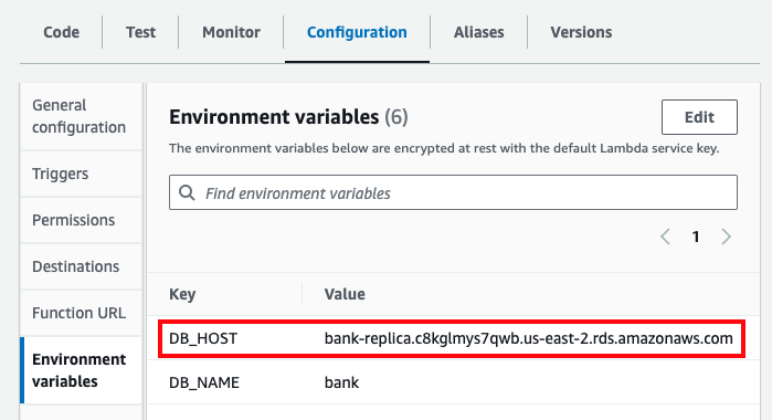
The Lambda function should now have the DB_HOST set to the replica’s URL, and not the primary’s. If everything looks
correct, test out the URL in the function_url output variable one more time:
$ curl https://<FUNCTION_URL>

{

  "result":[

    {"id":2,"name":"Karen Johnson","date_of_birth":"1989-11-18","balance":4853},

    {"id":3,"name":"Wade Feinstein","date_of_birth":"1965-02-25","balance":2150}

  ]

}
If you see the exact same results as before, congrats, that means your Lambda function is now reading data from a read replica! Moreover, your database is now backed up, both via the replica and daily snapshots.
|
Get your hands dirty
Here are a few exercises you can try at home to go deeper:
|
When you’re done testing, commit your code, and run destroy to clean everything up. Note that, as part of the
destroy process, RDS will take one final snapshot of the database, which is a handy failsafe in case you delete a
database by accident.
Conclusion
Let’s review some of the key takeaways from this blog post. Here are the first few:
-
Keep your applications stateless. Store all your data in dedicated data stores.
-
Don’t roll your own data stores: always use mature, battle-tested, proven, off-the-shelf solutions.
-
Use relational databases as your primary data store (the source of truth), as they are secure, reliable, mature, and they support schemas, integrity constraints, foreign key constraints, joins, ACID transactions, and a flexible query language (SQL).
These first few takeaways essentially boil down to one simple idea: your default choice for data storage should be a relational database. Maybe that sounds boring to you. Perhaps you’re itching to try that sexy new NoSQL database that you read about on Hacker News. It perfectly fits your use case! It’s so slick! It’s so fast and cutting edge! When it comes to data storage, cutting edge is typically a bad thing. Yes, cutting edge might get you access to new features, but what it really means is that you’ll also be the one to discover all the bugs, corner cases, missing features, lack of integrations, failure modes, and so on. What you typically want from a data store is that it’s reliable, predictable, and stable. This is the opposite of cutting edge. It’s boring. But when it comes to data storage, boring is good, and you should choose boring technologies.
That doesn’t mean you should never use other data stores. But you should only use them if you have use cases that a relational database can’t handle, which means you need to understand what these other data stores are good at—and what they are not good at. The next several key takeaways from this blog post cover the typical use cases for other types of data stores:
-
Use key-value stores to cache data, speeding up queries and reducing load on your primary data store.
-
Use CDNs to cache static content, reducing latency for your users and reducing load on your servers.
-
Use file servers and object stores to serve static content, allowing your app servers to focus on serving dynamic content.
-
Use document stores for semi-structured and non-uniform data, where you can’t define a schema ahead of time, or for search, when you need free-text search, faceted search, etc.
-
Use columnar databases for time-series data, big data, fast data, data warehouses, and anywhere else you need to quickly perform aggregate operations on columns.
-
Use message queues to run tasks in the background, with guarantees that tasks are completed and executed in a specific order.
-
Use event streams to build highly-scalable, decoupled, event-driven architectures.
In addition to these use cases, you may need to pick your data store based on scalability and availability requirements, per the following key takeaways:
-
Use replication and partitioning to make relational databases more scalable and highly available.
-
Use NoSQL and NewSQL databases when your scalability and availability requirements exceed what you can do with a relational database—but only if you can invest in the time and expertise of deploying and maintaining a distributed data store.
Finally, whatever data store you choose, keep the following key takeaway in mind:
-
Ensure your data stores are securely backed up to protect against data loss and data corruption, protect your backups, test your backup strategy regularly, and follow the 3-2-1 rule.
Let’s now move on to Part 10, which is all about how to monitor your systems, including logs, metrics, and alerts.
Update, June 25, 2024: This blog post series is now also available as a book called Fundamentals of DevOps and Software Delivery: A hands-on guide to deploying and managing software in production, published by O’Reilly Media!
